ECMT 6002/6702: Econometric Applications Week4 Tutorial

Hello, dear friend, you can consult us at any time if you have any questions, add WeChat: daixieit

ECMT 6002/6702: Econometric Applications

1    Practice problems

1.  Consider the following linear regression model:

y t = β1 + β2x2t + β3x3t + ut,    t = 1, . . . , 100.

In the matrix form, we have

y = Xβ + u.

(i)  Obtain the variance of the OLS estimator under the assumption that Var(u) = σ2 I.

(ii)  Obtain the variance of the OLS estimator when

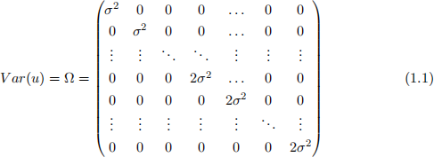
(iii) Explain what will happen in the standard t-test to examine H0  : β2  = 0 if you ignore potential heteroskedasticity.

(Optional) In this case, can you show that V ar(β bj ) is bigger than that under the as-sumption V ar(u) = σ 2 I?

- sumption Var(u) = σ2 I?

- Hint X′ AX is nonnegative definite if A is a diagonal matrix with nonnegative entries.

(iv)  Implement White’s heteroskedasticity test with 5% significance level. What is the aux- iliary regression equation?  Suppose that T  = 60 and TSS  =  1050, ESS  = 405 and RSS = 645 are obtained from the auxiliary regression.  Let A be the test statistic, B be the relevant critical value and C be defined by

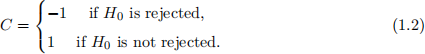
Find the value of A + B + C.

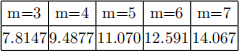
(Note) 95% quantile of χ2 (m)

2.  Consider the following regression model

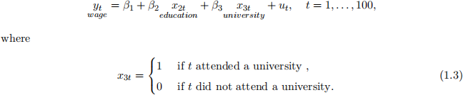
We want to examine if the variance of ut  gets larger along with the variable x3t

(a)  Explain how to implement the Goldfeld-Quandt (GQ) test in general (ignoring the prop- erty of x3t).

(b)  In order to example the hypothesis of interest using the GQ test, suppose that we split the samples into two subsamples of sizes T1  and T2  according to the variable x3t. Is this a reasonable approach? Why or why not?

2    Empirical application

We will consider the ECONMATH dataset again.  Suppose that we have the following regression model:

Instructions:

1.  The dataset contains missing values (see Week 3 tutorial)

2. Compute the OLS estimates and report their standard errors. In R, summary(lm(y ∼ X)) can be used if X is the (T × 5) data matrix.

3.  Implement White’s heteroskedasticity test and report the test result.  If things are correctly done, you can detect heteroskedasticity; more specifically,

TR2 ≃ 64                                                      (2.1)

and 95% quantile of χ2 (13) is 22.36 (why is the degrees of freedom parameter is 13?)

4.  Obtain the  heteroskedasticity-robust standard error  (i.e.,  White’s  standard error) of each coefficient estimate.   One easy way to do this in R is using“vcovHC”function given in “sandwith”package; specifically, run vcovHC(lm(y∼X)). Then obtain the t-statistics to examle H0  : βj  = 0.  The results must be simiar to

5.  Compare the above results with what you obtained using the usual standard errors in Week 3 tutorial.

6.  Obtain the HAC robust standard error of each coefficient estimate. In R“vcovHAC”func- tion given in“sandwith”package can be used; specifically, run vcovHAC(lm(y∼X)). Then obtain the t-statistics to examle H0  : βj  = 0.  The results must be simiar to

7.  This computing exercise is not mandatory. In this example, heteroskedasticity