115.109: Topic 1 Lab Worksheet: 'Tour de NZ' / Sustainability

115.109: Topic 1 Lab Worksheet: 'Tour de NZ' / Sustainability

{This is a replica of the instructions in the Excel sheet – so you can track through the instructions without having to jump around so much within Excel. Complete your answers within the Excel sheet, not here.}

Rationale Lab 1:

This first lab uses two different analytics problems (plus two more in Lab 2 - see the second tab at the bottom of the sheet).

First, we look at Gross Margin, and the impact of GST and discounts on margin calculations. These are pretty basic but fundamental concepts that are the core to retail business profitability. It is vital that retail staff know the difference between margin and markup, and understand how discounts affect the quantity sold required to maintain the same profit contribution.

Second, we consider a sample of consumer attitudinal data from a survey in New Zealand, collected in 2020.  This is a survey dataset about sustainability attitudes, intended purchase behaviours, and knowledge of and support for retailer sustainability practices. We will use this dataset in several of the labs, and in the Report. For Lab 1 we will look at a small part of the dataset, both in questions (columns) and respondents (rows)

We start by doing some basic data checking and manipulation: parsing and concatenation (splitting and joining cells).

We will also do some summary statistics (frequencies), using the CountIf function in Excel. More advanced students could use PivotTables, but we will use that tool in a future lab.

Task 1: (This Task is easiest read within Excel due to the many hints provided)

This bike is a "classic seller" for the "classic rider". It sells for RRP

$439.99

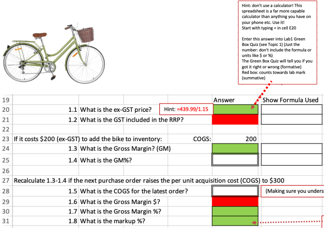
NB: the Green boxes are cells you can enter in the “Lab 1 Green Boxes Quiz (formative) Quiz. These don’t count for marks, but can be used to check you are doing it right. Once you’ve completed all the answers to the Quiz you will be told if you got the answer right or wrong (but not what the right answer is – so you can try again).

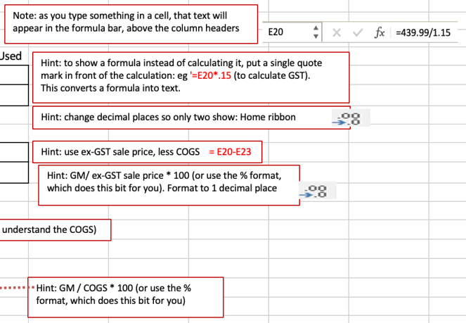
Additional Hints:

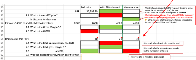
Task 2: (likewise easiest read in Excel)

A second model is added, an "e-bike" fully-suspended mountain bike with battery-powered assistance.

It has an RRP of $6999.99, but has a 20% 'launch' discount.

{NB: To temporarily show the various notes within Excel, hover mouse over the red triangle within Excel, or right-click a cell with a note and choose Show/Hide Note to show it permanently}.

NB: the Red boxes are cells you can enter in the “Lab 1 Red Boxes Quiz (summative)” Quiz. These DO count for marks, so you won’t know at the time if you have got the right answer, and you cannot  repeat it. You should also submit the whole spreadsheet (both Labs 1 & 2 answers completed), once    you’ve also completed the Lab 2 Red Boxes Quiz.

Task 3: Using the "SustainabilityData-10%sample" datasheet, do some data checks

This is a 10% subsample: a selection from a larger dataset, which we will use in future labs (and in the report).

For now, we need to check all data is OK (no missing data), and transform column B

Process:

1) Do the following in the SustainabilityData- 10%sample tab at the bottom of the spreadsheet

2) Use the quick scrolling keys to go the bottom and right of the dataset: holding the Cntrl

key (Windows) or Command key (Mac) and press the down arrow key to go the bottom of an 'array' (contiguous set of data)

Hold the Cntrl / Command key (Windows/Mac) and press the right arrow key to go the far right of an 'array' (contiguous set of data).

NB: if there are any breaks in the data, the highlighted cell (the one shown at the top of the spreadsheet) will stop just before the break. Check there are no breaks anywhere in the data

3) We need to remove the 'sec' (for seconds) that is in column 2. We could select the column and use Find > Replace (Find=" sec", Replace =""), or we could Parse the data.

Parsing means splitting data. We want to Parse the data in cells B5:B171 so that the number remains in column B, and the " sec" goes into column C (and could then be  deleted).

4) Select the data from cells B5:B108, by clicking in cell B5, then hold the

Control/Command + Shift and the down arrow key. (Holding Shift selects as you scroll.) 5) With the selected data, choose the 'Text to Columns' button on the Data toolbar (or for

Macs, also in the Data menu)

It offers two options: Delimited (where a specified character separates data) or Fixed Width. Choose Delimited, and click Next

Then select the Space option (you can leave the Tab option ticked - it makes no difference to this data), and Next

Finally it asks where to put the data; the default is fine (B5 onwards - note it will split the column into two, and spill into C5:C108 - since this is blank, that's all good)

6) The result is time data in column B, and 'sec' in column C, which we could remove. Instead, let's do the opposite action: Concatenation

Concatenation means linking together. There is the CONCAT function, but it is simpler to use a formula. In SustainabiltyData cell D5 enter the formula =B5&" "&C5

The & tells Excel that you are adding something to the contents of cell B5; the " " means you want a single space, and then the contents of cell C5.

The result is text, which you could then Parse using the Text to Columns function again … Instead, we are going to transform the contents in Column B with a formula: converting

seconds to minutes.

NB: this involves writing over what you have just done in column D. Don’t worry about it – you do not need to show the result of the concatenation.

7) In Cell D5, enter the formula =B5/60, to convert seconds to minutes. Format the result to    have a single decimal place. [We can only do this once we’ve removed the “ sec” text, and the cell converts from text to number format.]

Copy down, the quick way: copy cell D5, use the left arrow key to go to cell C5, then control/command+down arrow to go to cell C108. Right arrow to cell D108.

Now hold Control/Command+Shift+Up arrow to select the range D5:D108. Keep holding the Shift key (only), and press Down arrow once; you should now have D5:D108 selected. Paste (Control/Command+V)

(Alternatively you could drag down with the drag handle in cell D5.    It's much

8) Now Sort the dataset by Column D, in descending order (largest to smallest). Select D5:D108, and press Shift+Spacebar to select the entire rows.

Select Sort from the Home or Data ribbons (or the Data menu for Macs), and choose Largest to Smallest for column D

Depending on which method you choose, you may see the Sort dialog box, or three

options only

(choosing Custom List… brings up the dialog box).

NB: if you only selected column D, Excel would prompt you to Extend the range - but best to select all the data first.

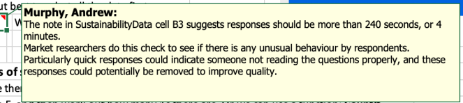
9) Interpret the result: are there any unusually long or short completion times?

Task 4: Using the "SustainabilityData-10%sample" datasheet, get frequencies of some demographic data

1) Determine the gender composition of the survey respondents. In cell E4, we can see there are three options: 1=Male, 2=Female and 3=Gender diverse (eg transgender, intersex)

To determine how many males we have, we could sort the whole dataset by column E, and then work out how many 1s there are. Or we can use a function: CountIf

2) In cell E110 (SustainabilityData sheet) enter the formula =COUNTIF(E5:E108,1), which counts how many cells in the range above contain a "1".

3) Copy the formula in E110, and paste in E111. Note what happens: because you have gone down a row, Excel changes the range accordingly [=COUNTIF(E6:E109,1)]

4) To correct this, in E110 add $ before the row numbers [ =COUNTIF(E$5:E$108,1)] and copy and paste again to E111, and E112

The $ anchors a cell reference: in front of a letter, it fixes the column; in front of a number, it fixes the row. (You can fix both at the same time if you wish.)

5) Now change the ,1) in E111 to ,2); and in E112 to ,3), to find how many 2s and 3s there are.

6) Copy and paste the results here - but because this table is formatted differently, you need to Paste Special

Copy cells E110:E112 from the SustainabilityData- 10%sample sheet, and in cell B110

below, right-click and choose Paste Special > and locate the Paste Special entry (not any of the pre-formatted options)

In the Paste Special box, select Values and Transpose

{The #DIV/0! error message means there is a formula in the cell that cannot be resolved, since it refers to a blank cell (the row above). When you paste information into

B110:D110, and complete the Sum in E110 [=sum(B110:D110)], the % formula should show the correct result. Check it to make sure!}

7) Now do the same for columns H, I and J of the SustainabilityData sheet. These are

'dummy' variables, where the answer options are either selected or not. In column H this is a 2 (if seelcted) or blank; in column I a 3 or blank; in column J a 4 or blank..

For now, calculate how many respondents selected these options in cells H5:H108, I5:I108 and J5:J108, into cells H114:J114 in the SustainabilityData sheet. Copy and Paste Special  > Values and Transpose those answers below.

NB: You can use =countif(range), using 2 as the criteria and selecting the cells to count as the range (eg =countif(H5:H108,2)