Information systems theory Tutorial 3

Objectives and organisation of tutorials:

•    Students will complete excel activities (including watching LinkedIn Learning videos) and case study readings prior to the tutorial

•    Students will work together to confirm their understanding of excel topics

•    Tutors will lead discussions on theoretical topics using the case study readings

•    Students will participate in quiz sessions to help reinforce learning. These quizzes are not assessed but the highest-ranked students will receive a prize at the end of the semester.

•    Students are strongly encouraged to attend all tutorials and take comprehensive notes. In  cases where a student cannot attend a particular tutorial, the student can complete the pre- tutorial activities on their own, watch the recordings, or follow up with the tutor during    consultation sessions.

Information systems theory

Read the case study ‘Japan Embraces E-government Tools for Tokyo 2020’ on Page 80-81 of the course text. Answer the four questions.

1a. Describe the identity verification system and describe the inputs, business processes, and the outputs of the system.

1b. Discuss how these IT applications strengthen the relationship between citizens and their government.

1c. What are the implementation challenges of these systems? How can they be addressed?

1d. What people, organization, and technology factors contributed to development of these IT applications?

Excel

Watch the following Excel videos (click on the links).

1. Freezing and unfreezing panes (5 minutes)

2. Splitting screens horizontally and vertically (5 minutes 20 seconds)

3. Collapsing and expanding data views with outlining (6 minutes 22 seconds)

4. Displaying multiple worksheets and workbooks (9 minutes 44 seconds)

5. Renaming, inserting and deleting sheets (4 minutes 13 seconds)

6. Moving, copying, and grouping sheets (6 minutes 7 seconds)

7. Using formulas to link worksheets and workbooks (8 minutes 57 seconds)

8. Locating and maintaining links (6 minutes 50 seconds)

9. Creating charts(optional)                                                (6 minutes 45 seconds)

10. Exploring chart types(optional)                                     (9 minutes 53 seconds)

11. Formatting charts(optional)                                            (7 minutes 12 seconds)

12. Working with axes, titles, and other elements(optional)(6 minutes 25 seconds)

13. Creating in-cell charts with sparklines(optional)        (7 minutes 16 seconds)

14. New charts in Excel 2016(optional)                            (10 minutes 19 seconds)

Note: ‘Optional’ videos are not assessed, but they are useful for the development of your Excel skills.

Files for this tutorial:

● 08 - Worksheet Views.xlsx

● 09 - 01 - EmployeeTable.xlsx,

● 09 - 01 - Home Product Line.xlsx

● 09 - 01 - RegionalSales.xlsx

● 09 - 02 - RegionalSales.xlsx

● 09 - 03 - RegionalSales.xlsx

● 09 - 04 - EmployeeTable.xlsx

● 09 - 04 - RegionalSales.xlsx

● 09 - 05 - EmployeeTable.xlsx

● 09 - 05 - RegionalSales.xlsx

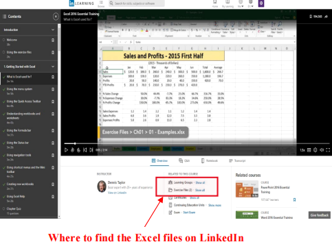
The files are available on Blackboard (under Learning Resources > Week 4 > Tutorial Resources) or on the LinkedIn site (see image below).

Organizing your worksheet view in Excel (workbook: 08 - WorkSheet Views)

1.   The freezing of panes is a very handy Excel feature (demonstrated with the worksheet “Freezing”). The Freeze Panes option is in the “View” tab of the Excel Ribbon. This option allows us three capabilities: Freeze/Unfreeze Panes; Freeze Top Row; Freeze First Column. Become familiar with always displaying a heading or a first column or freezing panes so that we can always see the top row AND an arbitrary number of left columns in our worksheet.

2.   Splitting the screen (demonstrated with the worksheet “SplitScreen”) left-right, or top-bottom, or four-way splits. The first two of these features are very handy and frequently used in large worksheets (not so the four-way split).

3.   Collapsing (and later expanding) detail is always very practical when we want to present data with an explanation of how it is constructed. This is demonstrated in the worksheet “Outlining” . In “Outlining”, we are presenting a budget, and this budget comprises monthly data that is then totalled (with the appropriate formulas both vertically and horizontally) on a Quarterly basis.

4.   Students should work through this worksheet (with the assistance of the video) to see how various levels of this data may be shown/hide. This involves the Excel feature “Outlining” that enables us to collapse (and expand) data by clicking buttons. This is achieved via the Data tab, then Group drop-down button (on far right of ribbon), and finally Auto Outline. Students should work through this capability – it is frequently used.

Displaying multiple worksheets and workbooks (workbooks: 09 - 01 - Home Product Line.xlsx;

09 - 01 - RegionalSales.xlsx; 09 - 01 - EmployeeTable.xlsx)

1.   Open the three workbooks/files. Now we have multiple files (3) open – and we frequently need to switch back and forth within these multiple files. We can see which files are open via the “View” tab and the “Switch Windows” button (this will show all open Excel files with the onscreen file ‘ticked’). We can use this display to switch from one file to another.

2.   If we are back in another tab, we lose the “Switch Windows” button, so (like any other button) we can add this to the “Quick Access” toolbar by right-clicking and adding (later deleting if appropriate).

Renaming, inserting, and deleting sheets (workbook 09 - 02 - ReginalSales.xlsx)

1.   We can easily rename sheets – either ‘right-click’ and rename, or ‘double-click’ the sheet name.  We can have spaces in a sheet name without a problem, and up to 31 characters to form the sheet name.

2.   We can ‘right-click’ to insert new sheets or to hide an existing sheet (unhide by again ‘right-clicking’ and choosing the sheet to unhide – consequently we should not use this capability for security – there is a better way that we shall look at later).

Moving, copying, and grouping sheets (workbook 09 - 03 - RegionalSales.xlsx)

1.   Move sheets by dragging the relevant tab (no commands needed). Make a copy of the sheet (to the existing workbook or a new workbook) by ‘right-clicking’ and choosing the appropriate action on the menu.

2.   We can also select multiple sheets (for example, East, South, Midwest and Pacific in the work  file). We do this by clicking one of the ‘end’ sheet tabs in our group, then hold down the ‘shift’ key and click the other ‘end’ sheet tab. When we have done this, we get the word ‘group’ appearing in the file name at the top of the screen, and we should know that any change in a selected sheet will also be made in all the other sheets in the selected group (e.g. insert a new row).

3.   We can ‘ungroup’ the tabs, by either ‘right-clicking’ a tab of the group (and selecting ‘ungroup’) or clicking a tab of a non-grouped worksheet.

Using formulas to link worksheets and workbooks (workbooks 09 - 04 - RegionalSales.xlsx and 09 - 04 - EmployeeTable.xlsx)

1.   Open both workbooks. In the worksheet RegionalTotals, in cell B2, we want a formula to add the contents of cell F3 in the East sheet, cell F3 in the Midwest sheet, cell F3 in the South sheet, and  finally cell F3 in the Pacific sheet. Notice how the formula appears in the formula bar, and the     role of the exclamation mark/point in this formula (as a separator between sheet name and cell reference). Notice the change in the formula if we change one of the sheet names to include spaces. This now means that the new sheet name (with a space) appears in single quotes in our     new formula (=East!F3+’Mid west’!F3+South!F3+Pacific!F3).

2.   Now move on to build a formula that adds the contents of cells in another file and worksheet (e.g. 09-04 - EmployeeTable.xlsx). In the resulting formula, notice again the use of the exclamation point/mark, but also the square brackets to enclose the workbook name. Notice that we finally end up with a complicated reference that includes the folder address of the other file – this can be a problem if we move workbooks.

Locating and maintaining links (workbooks 09 - 05 - EmployeeTable.xlsx and 09 - 05 - RegionalSales.xlsx)

1.   As demonstrated in the relevant video, build a formula in cell J5 of the ‘Furniture Sales worksheet of 09 - 05 - EmployeeTable’ workbook that references cell B7 in the ‘09 - 05 - RegionalSales’ workbook (“Summary” worksheet). Take note of the formula appearance. Take note of the Data   tab-> Queries and Connections group1->Edit link button. This button is greyed out in the source    workbook (‘09 - 05 - RegionalSales’, however it is active in the workbook ‘09 - 05 - EmployeeTable’ .