关键词 > Excel代写
Advanced Excel – Topic 2
发布时间:2023-07-11
Hello, dear friend, you can consult us at any time if you have any questions, add WeChat: daixieit
Advanced Excel – Topic 2
• Working with Multiple Worksheets: Grouping
• The LOOKUP function
Grouping multiple worksheets
Excel allows you to select multiple sheets, which you can then edit as a group, at the same time. This saves time and promotes a uniform appearance across all worksheets . This feature depends on identical positioning of data across all worksheets.
Tip: Take care to ensure the data you enter is accurate – or the error will appear on all worksheets!
Grouping also allows consolidation of data. You can refer to the same cell (or range) on multiple worksheets in formulas. This is called a 3D-reference.
Activity 2a – Grouping worksheets
1 Create a new workbook and save it as ToyShop.xlsx
2 Name four sheets: Jan, Feb, Mar, and QtrTotal.

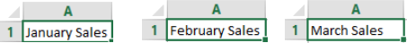
3 Enter different information in cell A1 for each of the 1st three sheets as shown below
- you will have to open each sheet separately.
4 In cell A1 of the QtrTotal sheet, enter the heading, First Quarter. 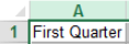
5 Group all sheets
a Click on the first sheet, Jan, hold down the Shift key while you click on the tab
for the last sheet, QtrTotal.
Holding down the Shift key when clicking on the first and last worksheet tabs automatically selects the worksheets in between the first and last.
The Ctrl key allows you to specify multiple worksheets if they are NOT next to each other.
Therefore, if you wanted to select just Jan and Mar, you would click the Jan tab, hold down Ctrl and then click the Mar tab. On a MAC, use the Cmd key instead of the Ctrl key.
You know the sheets are grouped when you can see a single line under all the grouped sheets at the bottom, and you can see the word [Group] in the Title Bar at the top of the Excel screen.

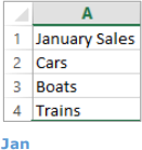
b Starting in cell A2, enter the information Cars, Boats, Trains in column A. Because the sheets are grouped, the information will appear on all the sheets.
6 Ungroup all the sheets by clicking on just one of the other sheets, or right click a sheet tab and choose Ungroup . Check that [Group] no longer appears in the Title Bar.
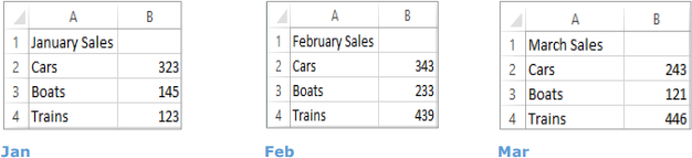
7 Enter different sales figures for each of the months on the separate monthly sheets as below. Do not enter figures in the QtrTotal sheet.
8 Group all the sheets again.
9 Enter the word Total under the list of goods (cell A5). Make it bold.
10 Under the sales figures, AutoSum the column of figures.
11 Insert a row at the top of the sheet, and type in the heading Toy Shop. Merge and Centre A1 and B1 and apply bold formatting .
12 Format the spreadsheet .
13 All the sheets will reflect these changes.
Consolidate the 3 worksheets using 3-D references
1 Select only the QtrTotal sheet.
2 In cell B3, click on AutoSum. You will see =SUM() in the cell .
3 Click on the Jan sheet, hold down Shift and click on the Mar sheet.
4 Click in B3 and press enter. In the QtrTotal sheet, the formula should be

5 Fill this formula down the column. This calculates the values from all the month sheets and displays the total in the QtrTotal sheet.
6 Save your file.
Activity 2b – Grouping practice
![]() Use the file Coffee Sales.xlsx for this activity.
Use the file Coffee Sales.xlsx for this activity.
This workbook contains 5 worksheets; one for each quarter of the year and a fifth which will be used to show the Year total by consolidating information from the 4 quarters.
1 Use grouping to make the following changes to all 5 worksheets:
a A3 in all worksheets has a spelling error. Correct Randwix to Randwick b A6 in all worksheets has a spelling error. Correct Naroubra to Maroubra c Add a label in A9 – Total and in A10 - Average
d Change the font of cells A2:F10 to Calibri 12.
e Bold and right align column headings in Row 2 (select the entire row)
g Format the title. Change font to Arial Black, 12
2 Ungroup the sheets and then use grouping to make the following changes to the Qtr1, Qtr2, Qtr3 and Qtr4 worksheets :
a Format the title : merge between A1:E1, and apply grey shading. b Add the label Total in E2
c Insert formulas in cells E3:E8 and B9:D9 to add the appropriate values.
d Insert formulas in B10:E10 to show averages for the appropriate values. Format
values in Row 10 with 2 decimal places
3 Ungroup the sheets and complete the Year Total worksheet:
a Add appropriate formulas to B3:B8 to consolidate the totals from each of the
4 quarters.
b Insert appropriate formulas in cells B9 and B10
4 Save your file.
Activity 2c – Further grouping practice
![]() Use the file StoreData.xlsx for this activity.
Use the file StoreData.xlsx for this activity.
StoreData contains four worksheets with earnings from four different duty-free stores in Sydney, and a Summary Sheet where you are required to consolidate earnings for these stores.
On the Summary sheet:
1 Copy and paste the months and column headings for each category.
2 Design formulas to total the sales from all four stores for every category of items for each month.
3 Insert a column, labelled Monthly Total, and insert a formula to calculate the total for each month.
4 Add a column with the heading Taxable .
5 There is a tax each month if Liquor sales are greater than $1,000,000 and Electronics sales are greater than $1,300,000.
Enter a formula to check for both of these conditions, showing the words “Tax to be Paid” if they are both true, and leaving it blank if not. Use absolute referencing.
6 Add a column with the heading Tax.
7 Enter a formula to show the amount of tax to be paid. This is 10% of the Monthly Total, but only payable on the amount above $5,500,000.
8 Finally, calculate the grand total earned after tax has been paid .
9 Format appropriately and save your file.
The LOOKUP function
You have already learned how to construct and apply the VLOOKUP and HLOOKUP functions.
Remember: VLOOKUP always looks in the leftmost column of a table and HLOOKUP always looks in the top row of a table.
LOOKUP can be used when the data arrangement doesn’t allow a VLOOKUP or HLOOKUP.
Activity 2d – Constructing the LOOKUP function
![]() Use the file Metals.xlsx for this activity.
Use the file Metals.xlsx for this activity.
Different metals require different amounts of energy to extract from their minerals.
In this spreadsheet, column C shows the amount of energy (kJ) required to produce 1 kg of metal from the specified mineral, and column D shows the amount of energy needed to produce any quantity of metal from its ore.
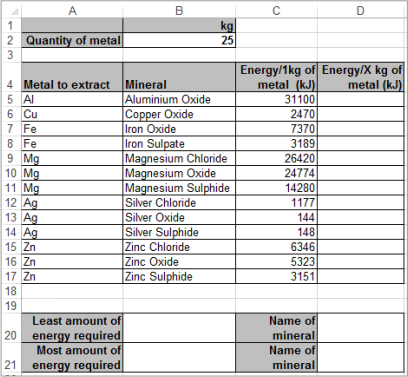
1 Sort* the data by the Energy/1kg of metal (kJ) column, smallest to largest.
2 In column D (Energy/X kg of Metal (kJ) use an absolute cell reference to calculate how much energy is required to extract 25kg of each metal .
3 Change cell B2 to 16 . Your numbers in column D should all change.
4 Below your spreadsheet in a summary area, use functions to show the least and the most amounts of energy (kJ) required to extract a metal (use column D).
5 Use the Lookup function to find the name of the minerals which require the least and the most amounts of energy to extract metal from their ores.
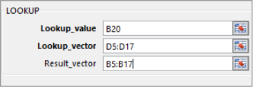
The formula should look like this:
=LOOKUP(B20,D5:D17,B5:B17)
|
*Note: The values in the lookup_vector (lookup range) must be sorted in ascending order, otherwise the LOOKUP may not give the correct value. |
6 Enter the following in the header: your name on the left, activity number and class in the centre and the date on the right.
7 Enter the automatic file name in the centre of the footer .
8 Format the worksheet to display the data effectively on one page.
9 Save your file.
Activity 2e – LOOKUP practice
![]() Use the file Car Parts.xlsx for this activity.
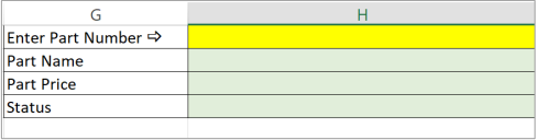
Use the file Car Parts.xlsx for this activity.
1 A user should be able to enter any Part Number into cell H1 (from the list in Column A)
2 Use appropriate functions to show:
a the corresponding Part Name in cell H2
b the corresponding Part Price in cell H3
c the corresponding Status in cell H4
3 Format and save your file.
Challenge
Activity 2f – Nesting IF and LOOKUP
![]() Use the file Flight Cost.xlsx for this activity.
Use the file Flight Cost.xlsx for this activity.
The data in this spreadsheet shows the cost of flights, and the star safety rating for each airline listed.
1 Create an area on the spreadsheet where you can enter the name of an airline.
2 Enter a formula that will return (display) “Don’t fly” if the Star safety rating for the chosen airline is lower than 7. If the rating is 7 or more, then display the cost of the flight.
Note: you will need to use a nested formula here.
3 Format and save your file.
