Simulating returns in Excel

Hello, dear friend, you can consult us at any time if you have any questions, add WeChat: daixieit

Simulating returns in Excel

Accompanying Excel file: Simulating returns in Excel.xlsx

Introduction

Why might you need to simulate returns? Consider a retirement planning problem with the following information:

Age now: 25

Projected retirement age: 65

Projected death age: 95

Desired monthly retirement income: $20,000

Expected return on investments: 8%

If you assume you earn an annual rate of 8% on your investments, then it’s a simple exercise (you certainly should try it! This is a simple time value of money exercise that every finance major or collateral should be able to do) to calculate that you’ll need to accumulate $2,725,670 in your retirement account by the day you retire, and you can do so by saving $780.77 a month from now until retirement.

But what if you don’t actually earn 8%? Some years you earn more, some years less. If you earn less, you’ll certainly accumulate less and you’ll run out of money before age 95 and be a burden on your family. Even if you wait until retirement to see how much you’ve accumulated and choose your monthly income based on that, your investment returns during retirement will vary and you, again, may run out of money.

So one question you’ll want to answer in your retirement planning is “given my level of contributions and my desired retirement income, what is the likelihood of running out of money?” Simulating investment returns can help you answer this question.

There are four steps in creating a simulation model

1. Create a model that depends on variables that you think will be random. In this case the random variables will be realized returns, but they could be inputs to a capital budgeting analysis, assumed post-acquisition performance of a company you are targeting for a merger, or even the financial outcome for an investment in exotic derivative securities!

2. Decide what random distribution your variables should follow and program Excel to feed these random variables into your model. We’ll use Excel’s probability distributions and inverse probability functions to accomplish this.

3. Program Excel to plug these random variables into your model many times (say, 1,000 or 10,000 times) and see what the result is for each of these “runs” is. We’ll use a data table for this step.

4. Evaluate the results of the simulation runs. For the retirement problem above, this might involve counting the percentage of times you run out of money before age 95. For a capital budgeting project, you might want to calculate the expected NPV of the project. 

I’ll address each of these steps in order, and then combine them into an example analysis.

Step 1. Create a model that depends on variables you think are random

I’ve created a sample model in the accompanying Excel file (Sample Models tab) that models a college savings plan in which a student (or family) saves up for expected tuition. There are 15 years of savings (one contribution at the beginning of each year) and 4 withdrawals, one at the beginning of each year of college. I plugged in the expected return for the actual return. I’ve also calculated the end of year investment account balance for each of the savings years and then each year once saving stops and withdrawals begin. By choosing a different level of savings, the user can end up with a positive or a negative balance after the final tuition payment. If the result is a negative balance, then there will be a shortfall—there won’t be enough in the account for the last tuition payment. If the result is a positive balance, then there will be money left over after all of the tuition is paid.

Step 2. Make your variables random

In the second section of the model labeled Simulation analysis, I assumed that annual stock returns are lognormally distributed with a mean of 8% and a standard deviation of 15%. What does this mean?

If r is an annual return, then we frequently approximate the distribution of y as lognormal with mean m and standard deviation s. This means that ln(1 + r) is distributed as a normal distribution (“bell curve”) with mean m and standard deviation s. You don’t need to know all the technical details about why this is an ok approximation, or under which circumstances this isn’t all that good an approximation. For our purposes, a lognormal distribution is good enough for simulating the investment/savings outcome.

Important note: if you want to simulate monthly returns rather than annual returns, then what m and s should you use? If your annual m is 8%, then your monthly m is 8%/12. That is, just divide the mean by the number of pieces you need. If daily, then 8%/252 (there are 252 trading days in a year!). But for standard deviation, you divide by the square root of the number of pieces! So if the annual standard deviation of returns is 20%, the monthly standard deviation will be 20%/sqrt(12) and for daily returns, it will be 20%/sqrt(252).

The way you do this in Excel is to use its inverse probability function. Given a probability, p, between 0 and 1, the inverse probability function gives the random variable associated with that probability. So we need a random number generator that generates numbers between 0 and 1, and then we plug that input into the Excel inverse probability function =LOGNORM.INV. See the Lognormal distribution tab in the attached Excel document.

The Excel formula for a single random annual return with mean 8% and standard deviation 20% is:

Random annual return  =LOGNORM.INV(RAND(),8%,20%) – 1

You have to subtract the 1 from the formula because we want r, not 1 + r.

You can type it in exactly like that, with the = sign. The RAND() function generates a new random number between 0 and 1 every time you make a change in your spreadsheet. Better yet, you should have a cell reference where the 8% is pointing to the cell where you put in your mean return, and a cell reference where the 20% is for the standard deviation.

If your desired mean return is in Cell A1 and your desired standard deviation is in Cell B1, then this would be your Excel formula:

Random annual return  =LOGNORM.INV(RAND(),A1,B1) - 1

I’ve plugged this formula into each year’s annual return cell in the model from Step 1. See the attached Excel spreadsheet.

Step 3. Plug in many times to run the simulation

If you wanted to run a simulation manually, you could take the model you created in Step 2 and simply press F9, say 1,000 times, and record the ending balance in your account and perhaps the average return over the 19-year simulation period with each press. Tabulate the data and see the number of times you ended up with enough money and the number of times you ended up with a shortfall.

That would, of course, take too long. Instead, we’ll use Excel’s data table feature to do that for us. If you already know how to create a data table and what they do, then skip this brief introduction to data tables and continue with the next section on using a data table to trigger a simulation.

A brief introduction to data tables

A data table is a way to get Excel to repeat something a bunch of times and record the answer. Usually, this involves plugging a bunch of different numbers into an input cell and recording the result of the calculation or output of the model for each different input. For example, suppose you have a spreadsheet model that is based on initial sales, which appears in cell B3, and the output of the model is NPV, which appears in cell B9.

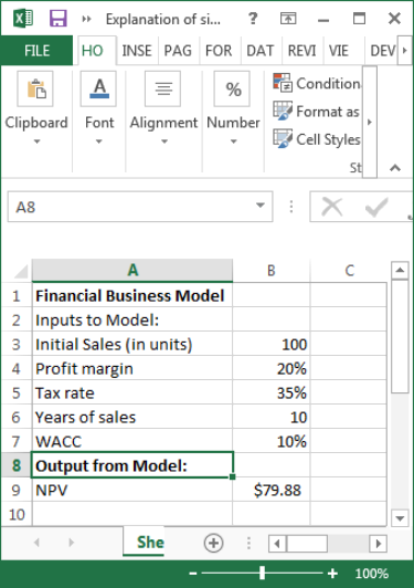
You could perform a sensitivity analysis by manually plugging different initial sales values into B3 and seeing how B9 changes.  Or, you could set up a Data Table to do the same thing automatically: choose a bunch of different initial sales figures, select Data/What if Analysis/Data Table and set the column input cell to B3, and get a summary of the resulting NPVs in the table.

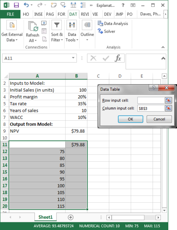
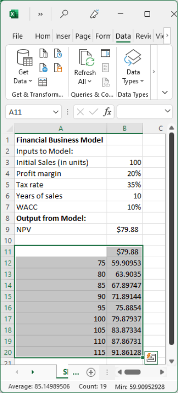
Cell B11 is just a cell reference pointing to the answer we care about, in this case =B9. When you highlight the region A11:B20 and click on Data/What if anlaysis/Data table and select the column input cell to be B3 and click OK, then Excel will run through the inputs in A12:A:20, that is the 75 and the 80 and the 85, …. And plug them into cell B3, and record the value that displays in B11 in cells B12:B20. It’s an easy way to conduct a sensitivity analysis.

Using a data table to trigger a simulation

In a simulation, we don’t want the data table to plug any values into an input cell. All we really want is for Excel to “press F9” a bunch of times to force a recalculation and record the output from our model each time.

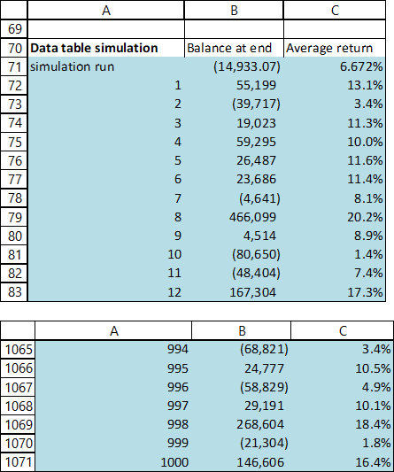
See the Sample models tab of the attached Excel spreadsheet. I’ve set up in the Data table simulation section the numbers from 1 to 1,000 to represent the number of “runs” I want to do.

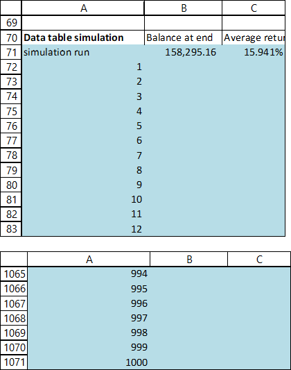
Cell B71 is just a cell reference pointing to the ending balance in our model after paying the last tuition payment from our model in Step 2. Cell B71 calculates the average of the 19 returns we simulated in Step 2.

Highlight A71:C1071 and click on Data/What if Analysis/Data Table and choose any unoccupied cell in your spreadsheet (A69 is a fine cell to choose) for the column input cell and press OK.  Excel will plug the 1, 2, 3, …. 1,000 into cell A69, which won’t do anything! Except that it will force a recalculation of all the random numbers you specified in your model in Step 2.

Note that I’ve set the spreadsheet calculation options to “Automatic except for data tables.” That’s to prevent the data table simulations from running every time you type anything into a cell (a simulation can take a long time to run. This one only takes a second or so on my computer, but longer run times can be irritating if you are working on your spreadsheet.). You can change this setting so that your data tables are recalculated (and therefore your simulation is re-run) every time you make any change in your spreadsheet by clicking on File/Options/Formulas/Calculation options and select Automatic instead of Automatic except for data tables.

Each time you hit F9, the spreadsheet will conduct another 1,000-run simulation of the model and record the portfolio balance after the last payment (or shortfall) and the average return over the 19-year investment period.   

Step 4. Evaluate the results of the simulation

How you evaluate the results of your simulation depends on the purpose of the simulation. If it is some sort of valuation or capital budgeting simulation, then perhaps you want to calculate the average value or average NPV that comes from the model. In this example, the question is whether or not you run out of money before you are done paying for college, so a natural variable to record is the portfolio balance after the last payment is made. If the balance is positive, then great! You have money left over after college! If it is negative, then that’s not good. It means you have a shortfall in your funding and you’ll need to come up with more money!

One way to do this is to plot a histogram that shows the range of ending portfolio values. I’ve also included the average portfolio return for each run of the simulation. See the attached file and the figures below.

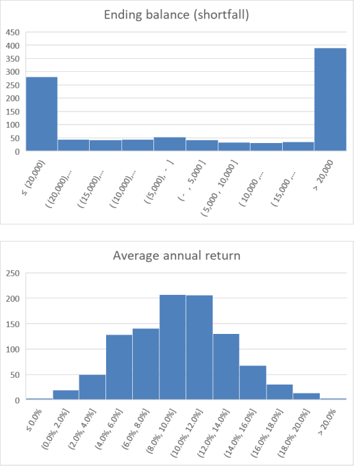
Notice that given the amount saved per year, you end up with a surplus about 40% of the time. But because the returns are quite variable (as are stock returns, in general!), sometimes you have a significant shortfall, and you end up needing an extra $20,000 or more to make it through school about 27% of the time!

How would this information help you? You could save more. That would shift the histogram to the right. Or you could invest some or all of the money in corporate or U.S. Treasury bonds instead of the stock market. Bonds have a much lower return, so you’d have to save more, but they have a lower standard deviation, so you’d get a more stable return.