FINM 3008/6016 Portfolio Construction Tutorial #3

Hello, dear friend, you can consult us at any time if you have any questions, add WeChat: daixieit

FINM 3008/6016 Portfolio Construction

Tutorial #3 – Outline

Background

During Lecture 3, we revised the concepts behind modern portfolio theory (MPT) and the mean-variance model (further details are provided in your week 3 supplementary readings). A central feature of MPT is the efficient frontier of risky assets. The efficient frontier extends from the minimum variance portfolio (MVP) and spans the asset weightings that provide the lowest risk for a given level of expected portfolio return (or the highest expected portfolio return for a given level of risk). This tutorial, we use the Excel add-in “SOLVER” to construct the efficient frontier, subject to various input assumptions and constraints. In the context of asset allocation, the portfolio weightings comprise the weights in each available asset class. The inputs to mean-variance optimization are the expected returns, variances and covariances of each asset class. Given that the true values of these inputs are unknown, they must be estimated (e.g. using historical sample means or models of expected returns). As you will see, the “efficient frontier” resulting from mean-variance optimization can be extremely sensitive to changes in these estimated inputs, as well as to changes in the constraints imposed on the optimizer (e.g. budget constraint, long-only constraint, maximum weighting constraint). The aim of the exercise in this tutorial is NOT producing asset allocation in practical use. Instead, it demonstrates how impractical the mean-variance optimization can be in solving real-world asset allocation problems.

In what follows, we will construct portfolios that have the lowest level of risk for a given return, subject to certain constraints and the distribution of expected returns. Through the use of the SOLVER add-in, we will estimate the efficient frontier as follows: we will minimise portfolio standard deviation, by choosing the weights of the risky asset classes subject to a) a fully invested portfolio (i.e. the budget constraint that all weights sum to one), b) any other constraints (e.g., we will include a long-only constraint in our analysis later on); and c) a given level of expected return (a single point on the frontier will be created for each specified return). Changing the given level of expected return will trace out dots along the estimated efficient frontier. (Note: the MVP can be computed by removing the constraint specifying a given level of expected return.)

Very important: This exercise assumes the investor’s only objective is to minimize portfolio standard deviation, subject to some constraints. By setting different objective functions, such as maximizing portfolio returns or maximizing Sharp ratio, the model will produce different output of the optimal portfolios (the shift of the efficient frontier). The analysis is conducted on monthly return indices, which assumes the portfolio performance is evaluated over monthly horizon. For most investors in the real world (eg., funds managers, mum and dad investors, retirees) their portfolios are evaluated over much longer horizons (eg. 3 years), as their investment horizons tend to be very long term.

This exercise is not designed to repeat what you have learned in previous finance courses (eg. running an optimizer based on Yahoo Finance data). Instead, students are expected to appreciate how such “naïve and simple” portfolio construction exercise is unrealistic and can be very wrong if we consider the real-world circumstances, specifically related to our discussions in week 2 and in more details in coming weeks. The aim of this exercise is to help students to form their own critiques on MPT and to deepen their understanding the science and art of applying classical finance theories in practice.

Question 1

On the course Wattle site can be found the file “Tutorial #3 Analysis File.xlsx”. This file contains month-end total return indices in A$ for nine asset classes, plus various half-completed worksheets and charts. You are to develop this file with a view to estimating efficient portfolios. This is the second in a series of learning-by-doing exercises with the objective of giving exposure to spreadsheet-based analysis of portfolios using real data, and preparing for the assignment.

The aim is to use the ‘Solver’ add-in in Excel to estimate the mean-variance efficient frontier of portfolios under the three conditions listed below. (Note: Search Excel Help on “add-ins” if you need to load Solver.)

(a) Unconstrained portfolios i.e. (short positions are permitted), with inputs based on historic data without adjustment.

(b) Long-only portfolios, with inputs based on historic data without adjustment.

(c) Unconstrained portfolios, with expected returns imposed, i,e. the mean return for each asset class is to be adjusted towards certain target compound expected returns. The target returns and associated monthly means for ln(1+R) can be found in the worksheet named ‘E(R) adjust’.

What is required:

· Provide the portfolio weights and other measures (means, standard deviations, Sharpe ratio) across the target return range shown in the ‘SUMMARY’ worksheet. Note: As the analysis is to be based on monthly returns, monthly estimates are the basic unit of account. Provision is made to report indicative annualized equivalents to aid in interpretation, as people tend to think in annual terms. This can be done by multiplying monthly mean returns by 12 and annualizing variance under the assumption that monthly returns are independent, both of which are rough approximations.

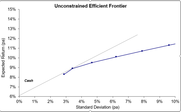
· Plot the efficient frontier (use a scatterplot – templates appear in the file), and the ‘capital market line’ from cash. This should touch at the tangent portfolio, which is the one with the maximum Sharpe ratio. Note that you should adjust the slope of CML manually to touch the efficient frontier and it should intersect with the vertical axis at the expected return of cash (in this exercise, we assume the average historical return of cash is the expected return). For instance, the unconstrained portfolio chart should look something like this:

Notes on this exercise:

· While the data file provides you with a template, you will need to understand the task at hand in order to develop the file to deliver the results. Be sure to examine the structure/formulas that already exist. The cells you need to complete are shaded light yellow (you will need to fill in the cells B2:K5 before you use SOLVER).

· Cash is left out of the optimization, as it will be treated in this instance as if it were a ‘risk-free asset’. The return on cash can be used as an indicative risk-free rate.

· The worksheets calculate the return on the ‘risky asset’ portfolio each month by referencing the vector of weightings in row 7. (Note: Applying the same asset class weightings every period assumes ‘monthly rebalancing’.)

· The analysis requires you complete the cells that estimate the mean and variance or standard deviation of portfolio returns, as well as the Sharpe ratio.

· The cells N11 through AB11 are designed as an area where the results appear, so that they can be copied as dead numbers into the cells in the rows below. You must enter the Sharpe ratio formula in AC11 yourself. The charts and summary sheet are linked to this section. Once you have completed the solver exercise, the “efficient frontier” proposed by the solver will appear on the chart (make sure you can replicate this yourself). You can then adjust the line extending from the cash rate so that it’s tangent to the efficient frontier at the point where the Sharpe ratio is maximized (the average historical cash rate of 6.25% p.a. is used as the expected cash rate. You will need to adjust the capital market line so that it reflects the expected cash return). This is approximately the hypothetical “efficient market portfolio” suggested by the optimizer.

· Solver is used to find the portfolio weight vector appearing in cells B7 to I7. (Note: to begin with, equal weights (12.5%) are entered in B7 to I7. This is because SOLVER needs a starting point, so these cells cannot be left empty. Note that there might be a few solutions to the problem but SOLVER only provides one solution every time you run it. You may expect to have different solutions from others, or have different solutions if you start with different initial weightings.)

· The first step is to find the ‘minimum variance portfolio’ weights by minimizing variance or standard deviation of portfolio returns (column J; e.g. portfolio variance = cell J3) , subject to the constraint that weightings sum to 1 (i.e. cell J7 = 1). Copy the results appearing in cells N11:AC11 to N13:AC13, pasting as values.

· Other efficient portfolios can be estimated by minimizing either variance or standard deviation subject to achieving various return targets. The blue cells near the top of columns M, N and O are set up to achieve this outcome. You will need to add a constraint that the difference between the target return and the portfolio return is zero, i.e. cell M4=0. To do this, you can use cell N3 to specify monthly return targets in excess of the minimum variance portfolio return (the analysis increases targets in steps of +0.05% upwards from the minimum variance portfolio return, towards a maximum of +0.35%), then include M4=0 in your solver.

· Correct portfolio returns and standard deviations appear in columns AD and AE. If you don’t get these, you have probably made an error.

· Repeat the entire process for long-only portfolios (‘Long-only’ worksheet) by including constraints that the cells containing weightings for each asset class are all  ‘>= 0’ and ‘<= 1’. (You may get away without the ‘<= 1’ constraint, although you may find that Solver will try to hold more than 100% of some assets when no feasible solution exists.)

· The ‘Adjusted E(R)’ spreadsheet includes series with the mean compounded return adjusted towards a target, in similar fashion to Tutorial #2. (Note: in purple are the expected (target) returns, which we will talk about more in Topics 4 and 5. Also note that unlike previous tabs, here we use compounded (log) as opposed to arithmetic returns, to illustrate both methods. The best method to use depends on the objective and circumstances, which will be discussed more in Topic 4.) Repeat the analysis here without any long-only constraints, but include a constraint that the weighting on direct property (cell F7) must be less than or equal to 10%. The reason for this constraint is discussed in week 2 lecture briefly and will be revisited in following weeks with more examples and details.

Discussion points

(a) Scrutinize the unconstrained weightings. What is the optimizer doing?

(b) Scrutinize the long-only weightings. What is the optimizer doing?

(c) The weightings arising from the mean-adjusted data seem to broadly make sense. What do you think is going on? Why was it necessary to constrain the direct property weighting? (See what happens if this constraint is not excluded.)

(d) To what extent is this type of analysis useful in identifying a portfolio you might want to hold in practice?   

Question 2

What are the key problems that arise from using traditional mean-variance portfolio optimization to set asset allocation in practice? (Please come prepared with a list of four (4) problems you have identified. The aim is to compile a list during the tutorial.)