COMP3308/3608 Artificial Intelligence, s1 2023 Weeks 5 Tutorial exercises

Exercise 1 (Homework). K-Nearest Neighbor with numeric attributes

A lecturer has missed to mark one exam paper – Isabella’s. He doesn’t have time to mark it and decides to use the k-Nearest Neighbor algorithm to predict Isabella’s exam grade based on her marks for Assignment 1 and Assignment 2 and the performance of the other students in the course, shown in the table below:

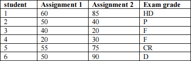
Isabella’s assignment marks are: Assignment 1 = 65 and Assignment 2 = 80. What will be the      predicted exam grade for Isabella using 1-Nearest Neighbor with Manhattan distance? Show your calculations.

No need to normalize the data, all marks are measured on the same scale – from 0 to 100.

Solution:

The last column of the table shows the Manhattan distance between the new example (Isabella) and the other students:

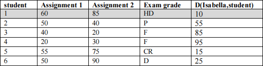
The closest neighbor (smallest distance) is Student 1 whose exam grade is HD => 1-Nearest-Neighbor will predict HD for Isabella’s exam grade.

Exercise 2. K-Nearest Neighbor with nominal and numeric attributes

The following dataset describes adults as short, medium and tall based on two attributes: gender and height in meters.

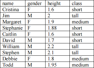
What would be the prediction of 5-Nearest-Neighbor using Euclidian distance for Maria who is (F, 1.75)? Show your calculations. Do not apply normalization for this exercise (but note that in practical situations you need to do this for the numeric attributes). In case of ties, make random selection.

Hint: gender is nominal attribute; see the lecture slides about how to calculate distance for nominal attributes.

Solution:

Gender is a nominal attribute, height is a numeric. When calculating distance for nominal attributes we can use the following rule:

difference = 1 between 2 values that are not the same

difference = 0 between 2 values that are the same

Maria: gender=F, height=1.6

D(cristina, maria) = sqrt(0+(1.6- 1.75)^2)=sqrt(0.0225) *short

D(jim, maria) = sqrt(1+(2- 1.75)^2)=sqrt(1.0625)

D(margaret, maria) = sqrt(0+(1.9- 1.75)^2)=sqrt(0.0225) *medium

D(stephanie, maria) = sqrt(0+(1.88- 1.75)^2)=sqrt(0.0169) *short

D(caitlin, maria) = sqrt(0+(1.6- 1.75)^2)=sqrt(0.0225) *short

D(david, maria) = sqrt(1+(1.7- 1.75)^2)=sqrt(1.0025)

D(william, maria) = sqrt(1+(2.2- 1.75)^2)=sqrt(1.2025)

D(stephen, maria) = sqrt(1+(2. 1- 1.75)^2)=sqrt(1. 1225)

D(debbie, maria) = sqrt(0+(1.8- 1.75)^2)=sqrt(0.0025) *medium

D(todd, maria) = sqrt(1+(1.95- 1.75)^2)=sqrt(1.04)

The closest 5 neighbors are Debbie, Stephanie, Cristina, Margaret, Caitlin. Of these 5 examples 3 are short and 2 are medium. Thus, 5-nearest neighbor will classify Maria as short.

Note: If there is a tie, the selection is random as the exercises says. For example, if there were 2 tall, 2 medium and 1 short, tall or medium would be selected randomly.

Exercise 3. 1R algorithm

Consider the iPhone dataset given below. There are 4 nominal attributes (age, income, student, and credit_rating) and the class is buys_iPhone with 2 values: yes and no. Predict the class of the following new example using the 1R algorithm: age<=30, income=medium, student=yes, credit-rating=fair. Break ties arbitrary.

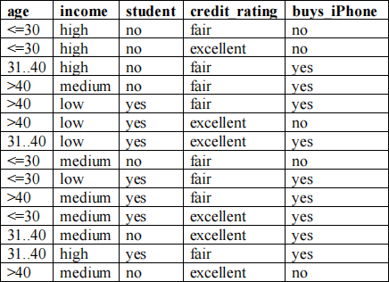
Dataset adapted from J. Han and M. Kamber, Data Mining, Concepts and Techniques, 2nd edition, 2006, Morgan Kaufmann.

Solution:

1. Attribute age

<=30: 3 no, 2 yes; age<=30-> buys_iPhone=no, errors: 2/5

31..40: 4 yes, 0 no; age = 31..40->buys_iPhone=yes, errors: 0/4

>40: 3 yes, 2 no; age>40->buys_iPhone=yes, errors: 2/5

total errors: 4/14

2. Attribute income

high: 2 no, 2 yes*; income=high-> buys_iPhone=yes, errors: 2/4

medium: 4 yes, 2 no, income=medium->buys_iPhone=yes, errors: 2/6

low: 3 yes, 1 no; income=low->buys_iPhone=yes, errors 1/4

total errors: 5/14

3. Attribute student

no: 4 no, 3 yes; student=no->buys_iPhone=no, errors: 3/7

yes: 6 yes, 1 no, student=yes->buys_iPhone=yes, errors: 1/7

total errors:

4/14

4. Attribute credit_rating

fair: 2 no, 6 yes, credit_rating=fair->buys_iPhone=yes, errors 2/8

excellent: 3 no, 3 yes*; credit_rating=yes->buys_iPhone=yes, errors 3/6

total errors: 5/14

*- random selection

Rules 1 and 3 have the same (minimum) number of errors; let’s choose randomly the first one => 1R produces the following rule:

if age<=30 then buys_iPhone=no

elseif age=31..40 then buys_iPhone=yes

elseif age>40 then buys_iPhone=yes

The new example age<=30, income=medium, student=yes, credit-rating=fair

is classified as buys_iPhone=no.

Note that rule 3 would classify it as buys_iPhone=yes.

Exercise 4. Using Weka

Weka is an open-source ML software written in Java and developed at the University of Waikato in   New Zealand, for more information see http://www.cs.waikato.ac.nz/ml/weka/index.html. It is a solid and well-established software written by ML experts.

Install Weka on your own computer at home, it will be required for Assignment 2. Meanwhile we will use it during the tutorials to better understand the ML algorithms we study.

1.   Get   familiar   with   Weka   (Explorer).   Load   the   weather   data   with   nominal   attributes (weather.nominal.arff). The datasets are in \Program Files\Weka-3.8.

2. Choose ZeroR classifier.

3. Choose “Percentage split” as ‘Test option” for evaluation of the classifier: 66% training set, 33% testing set

ZeroR is a very simple ML algorithm (also called “straw man”). It works as follows:

•   Nominal class (classification) – determine the most frequent class in the training data most_freq; classification: for every new example (i.e. not in the training data), return most_freq

•   Numeric class (regression) – determine the average class value in the training data av_value; classification: for every new example (i.e. not in the training data), return av-value

ZeroR is useful to determine the baseline accuracy when comparing with other ML algorithms.

4. Run the IBk algorithm (k-nearest neighbor, IB comes from Instance-Based learning; it is under “Lazy”) with k=1 and 3.

Was IB1 more accurate than IB3 on the test data? Does a higher k mean better accuracy? How does IB1 and IB3 compare with ZeroR in terms of accuracy on test set?

5. Consider IB1. Change “Percentage split” to “Use training data”(i.e. you will build the classifier using the training data and then test it on the same set). What is the accuracy? Why? Would you   achieve the same accuracy if IB1 was IBk, for k different than 1?

6. Now load another dataset – iris.arff. Run and compare the same algorithms. Don’t forget to normalize the data (the attributes are numeric). The normalization feature is under Filters-Unsupervised-Attribute- Normalise.

Why we didn’t normalize the weather data when we run IBLk above on the weather data?

Answer: The attributes were nominal; Weka calculates the distance as in exercise 2 (0 if the attribute values are the same, 1 if they are different) => all attributes are on the same scale, no need to normalize.

7. Select the K-star algorithm, another lazy algorithm, a modification of the standard nearest neighbor. Read its short description (right click on the algorithm’s name -> “Show properties’ -> “More”). Run it and compare the results (accuracy on test set using “Percentage split” again) with the 1 and 3 nearest neighbor algorithms and ZeroR.