关键词 > MATH3076/3976/4076
MATH3076/3976/4076 Mathematical Computing Semester 1, 2023
发布时间:2023-05-14
Hello, dear friend, you can consult us at any time if you have any questions, add WeChat: daixieit
MATH3076/3976/4076 Mathematical Computing
Semester 1, 2023
Project: Image Denoising
Due date: 11.59pm Monday 22 May (Week 13)
General Instructions
• Submit your report on Canvas as a single pdf file.
• Details about the report format and the grading are given at the end of this document.
• You are encouraged to work together on the project, but everything you submit—including code— must be your own work (i.e. write up independently). See Canvas for more information about
academic honesty.
This assignment is for MATH3976/4076 only. MATH3076 students should complete assignment 3.
Introduction
Mathematical models of images are a powerful set of tools for practical problems such as manipulating photos in Photoshop, medical imaging, security screening, and industrial quality assurance. In this project you will develop and implement mathematical models for image denoising: removing grainy noise from
images to get a cleaner, more realistic result. Some of the ideas from this project were used to improve the clarity of the first-ever image of a black hole in 2019 (Figure 1).
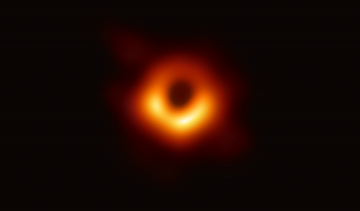
Figure 1: The first image of a black hole, from 2019 [Event Horizon Telescope collaboration et al].
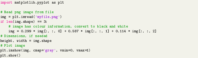
A digital black-and-white image is basically a matrix A ∈ [0, 1]m×n (for a 2D image that is m pixels high by n pixels wide) of pixel intensities in [0, 1], where 0 is black and 1 is white.1 A colour image is a ‘tensor’, A ∈ [0, 1]m×n×3, where the third dimension represents red, green or blue: every colour can be represented using different amount of these three colours.2 Perhaps surprisingly, one common way to convert a colour image to black-and-white is to take a weighted average of red, green and blue:
gray = 0.299 · red + 0.587 · green + 0.114 · blue.
The 1D version of an image is just a vector signal v ∈ [0, 1]n , like the sound waves shown in the Fourier
Transform lectures.
In Python, you can read a black-and-white or colour image into a NumPy array using matplotlib’s imread command, and display an image using imshow.![]()
I have included a collection of 6 example PNG files for you to use (see Figure 2). All images are 768 pixels wide and 512 pixels high.
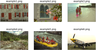
Figure 2: Example images, from https://r0k .us/graphics/kodak/.
I have also included a CSV file with 5 1D‘images’, each of length 1024 pixels. They are shown in Figure 3.3
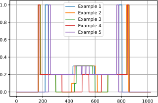
Figure 3: Example 1D images.
1D or 2D? You may use either 1D or 2D images (or both) for this project. However, working with the 2D
images is more complicated, and I will take this into account when grading. If using the 2D images, you should convert them to black-and-white first. For testing, you may want to use smaller images (i.e. fewer pixels) so your code runs faster.
Adding Noise
Since this project is about how to remove noise from an image, we need to be able to add noise to an image first. We can use our original image as a‘ground truth’, to test how good our noise removal is.
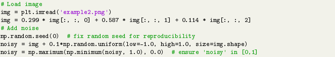
To add noise to an image, we can add a random perturbation to each pixel (and then making sure our pixel intensities are still in [0, 1]).
The resulting image is shown (compared to the original image) in Figure 4 below.
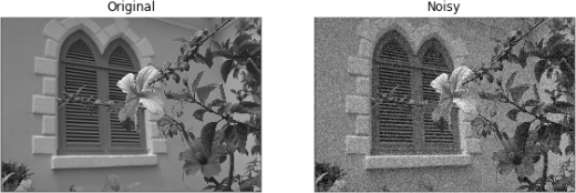
Figure 4: Example noisy image.
The same idea works for 1D images.
Denoising
To perform denoising, we first have to try and figure out a measurable property of‘noise-free’images. Given this property, we can then try to change a noisy image to have more/less of this property, which hopefully makes it look less noisy. There are many ways this can be done, but we will consider a common and important approach based on‘total variation’denoising.
If you look at many real-world images, they often have large regions of similar colours followed by sharp jumps to a different colour. For example, between the sky and the horizon in example 6 or between the bricks and the wall in example 2 (Figure 2). This means that a reasonable first model for ‘realistic’ images is piecewise constantfunctions.
How can we quantify how close to piecewise constant an image is? Thinking of an image as a function (of space), we want the gradient to be mostly zero, with a small number of places where it is nonzero.
Question 1. Given an image A ∈ [0, 1]m×n, we can think of this as a function of space, Ai,j = A(xi,yj) for a 2D discretisation (xi,yj) of the image domain. Derive an approximation for the gradients in the x and y directions ∇北A,∇yA ∈ Rm×n, where (∇北A)i,j is the approximate x-partial derivative of the image at pixel (i,j). (in 1D we only have ∇XA)
For a piecewise constant function, ∇北A and ∇y A should be mostly zeros. We could quantify this by counting the number of nonzero entries, such as
∥∇北A∥0 := # nonzero entries in |∇北A|, (1)![]()
(note this is often written as a norm even though it isn’t one). Mathematically, (1) is impractical to work with and instead we use an expression motivated by the ℓ1 norm for vectors:
m n
∥∇A∥TV := 工工 |∇xA|i,j + |∇yA|i,j ,
i=1 j=1
(noting the similarity to the ℓ1 norm to promote sparsity; see the data science lectures). So, smaller values of ∥∇A∥TV typically indicate a more ‘realistic’image. For 1D images, we can just use the ℓ1 norm directly.
Now, given a noisy image A, we want to find a denoised image ![]() . From the above, we expect two things:
. From the above, we expect two things:
• ![]() is close to A (since they are images of the same thing); and
is close to A (since they are images of the same thing); and
• ∥∇![]() ∥TV is smaller than ∥∇A∥TV .
∥TV is smaller than ∥∇A∥TV .
We can formulate this mathematically as an optimisation problem:
min ∥![]() − A∥F(2) + λ∥∇
− A∥F(2) + λ∥∇![]() ∥TV , (2)
∥TV , (2)
![]() ∈Rm ×n
∈Rm ×n
for some λ > 0, which captures the trade-off between the two goals. The Frobenius norm is used because it is just a quadratic function of the entries of ![]() .
.
This is a convex function of ![]() , but it is not differentiable, so the optimisation algorithms discussed in lectures do not apply. To cope with this, we can modify (2) to be a differentiable function via
, but it is not differentiable, so the optimisation algorithms discussed in lectures do not apply. To cope with this, we can modify (2) to be a differentiable function via
m n
![]()
![]()
![]()
![]() n ∥
n ∥![]() − A∥F(2) + λ 工工^|∇x
− A∥F(2) + λ 工工^|∇x![]() |i(2),j + |∇y
|i(2),j + |∇y ![]() |i(2),j + ϵ , (3)
|i(2),j + ϵ , (3)
for some ϵ > 0 (smaller means a better approximation to (2)). We could optionally apply bound constraints ![]() i,j ∈ [0, 1] if we wanted.
i,j ∈ [0, 1] if we wanted.
Question 2. Either implement a suitable optimisation algorithm for solving (3), or find a suitable algorithm to use in SciPy. Find suitable values for λ and ϵ that give you good results, and analyse how good your denoising results are. Discuss how your chosen algorithm would perform if the image size (number of pixels) increased dramatically.
Optional extension: a simple algorithm for solving (2) directly is proximal gradient descent. This comes from handling the non-differentiable term via a‘proximal operator’: it is easy to find online an expression for the proximal operator for a vector ℓ1 norm, for example. If you want, you could implement this algorithm instead (so you only have to find a good value for λ), but you would have to explain how this algorithm works.
Report/Grading
You should produce a written report outlining:
• The real-world problem to be solved.
• The model used to turn this into a mathematical problem.
• The algorithm(s) used to solve this problem.
• Your results (how did you find good values for λ and ϵ? how good are your final images?).
You should address the points mentioned in questions 1 and 2 above, but your document should be a standalone report (i.e. you shouldn’t write“the answer to Q1 is...”). I expect your report to be approximately 4–5 A4 pages with sensible font size and margins. You should include citations where relevant (e.g. if you look at proximal gradient descent); any reasonable format is acceptable.
Your report should not include code, only your mathematical work and results (including any images). You should include a copy of your code at the end of your report; this does not count as part of the the 4–5 pages.
Your report is worth 15% of your course mark. It will be graded based on:
• Completeness: is the problem and your model/methods fully explained? Did you interpret your results rather than just state them? Did you answer each question thoroughly?
• Mathematical correctness: mathematical reasoning is correct, efficient/elegant methods are used
• Writing: report is well-organised and easy to understand, graphs are properly formatted, spelling & grammar are correct, etc.
When I write journal papers, one question I use to check if I presented my work in enough detail is: could the person reading this (given sufficient time) completely recreate my results basedjust on what I have written?
The relative weight of each part of the report is as follows:
|
Report Part |
Marks |
Weighting |
|
Description of problem |
3 |
10% |
|
Development of model and algorithms |
12 |
40% |
|
Results & discussion |
12 |
40% |
|
Quality of presentation & writing |
3 |
10% |
|
Total |
30 |
100% |
