Simulation and Machine Learning Project

Simulation and Machine Learning Project

1 Pricing a Vertical Spread (25% of project credit)

1.1 Overview

A vertical spread is strategy whereby the option trader purchases a certain number of options at strike price K1 and simultaneously sells an equal number of options of the same underlying asset and same expiration date, but at a different strike price K2. We will consider a bull call spread for which the trader buys and sells call options with K1 < K2.

We consider that the underlying asset St follows geometric Brownian motion

where the risk-free interest rate r and volatility σ are constants. The initial condition is S0. Time t is measured in years. The payoff for the bull call spread is

where T > 0 is the time to maturity (or expiry).

The aim of Part I of the project is to price such a bull call spread by Monte Carlo simulations.

1.2 Particulars

Use the following parameters

1. The strike prices are K1 = £90 and K2 = £115 .

2. Time to maturity (or expiry), T, is 2 years.

3. The interest rate is r = 0.025.

4. The volatility is σ = 0.3.

You will want to price the bull call spread over a range of spot prices from S = £10 to S = £200.

1.3 Computational Tasks

● Write Python functions that computes the price and delta of a bull call spread directly from the Black-Scholes formula. These is will useful for testing your Monte Carlo simulations. These should be contained in a Python module (.py file).

● Implement the Monte Carlo method for pricing the bull call spread:

– Without any variance reduction (naive method);

– With antithetic variance reduction;

– With control variates;

– With importance sampling.

These functions, and the function that computes delta discussed below, should all be contained in a Python module (.py file). There should be sufficient comments within the module to explain the purpose of each function.

● With a moderate sample size, run naive Monte Carlo simulations (no variance reduction) for asset prices from S = £10 to S = £200 in steps of £5. From the variances of these simulations, determine a sample size such that the absolute accuracy of the Monte Carlo price is £0.01, with a 95% confidence level, over the full range of asset prices 10 ≤ S ≤ 200. For that sample size, price the bull call spread for S = £10 to S = £200.

Note: the variance depends on the value of S. Do not choose different sample sizes for each S. Choose a single sample size based on the maximum variance over the full range of S.

● Repeat what was done in the previous case for each of the three types of variance reduction.

● Using a method of your choice, implement an accurate computation of the delta for this option. You only need to do this for one of the variance reduction methods.

1.4 Report contents

See general discussion of report contents in Sec. 5 and 6.

● Explain, briefly, how you implemented the control variate and importance sampling methods. (It is not necessary that you explain naive Monte Carlo or antithetic variance reduction.) The goal is to make the report understandable independently of the Python module containing the main computational functions.

● Explain and justify how you determine the sample sizes to obtain the required accuracy. Plots might also be useful here.

● Plot option price as a function of spot price over the S studied. The various methods should give the same result. You may plot them on separate plots or on the same plot. You may also want to include the values obtained from Black-Scholes formula.

● Explain, briefly, your method for computing delta and justify why you chose this method.

● Plot of your solution for the delta together with values from the Black-Scholes formula.

● Compute and plot the option price and the delta for a variety of maturity times T and discuss. One possibility is surface plots of V (S, T) and ∆(S, T). (See example on Wikipedia page for the Black-Scholes model.)

● Finally, discuss the above results. You may discuss results from a financial perspective. Discuss briefly the pros and cons of the different numerical approaches. Discuss any improved efficiency from variance reduction.

2 Pricing a Barrier Option (25% of project credit)

2.1 Overview

A barrier option is a path-dependent option where the payoff depends on whether the underlying asset St hits or does not hit a specified barrier before expiry. Here we consider a down-and-out put option. This is a put option that becomes worthless if the asset price falls below the barrier Sb at any time between the present and expiry T. Hence the payoff is:

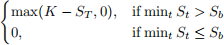
where K is the strike price.

For the underlying process we will use the geometric Brownian motion

allowing for the possibility that the volatility can depend on time and current value of underlying asset St. Below we refer to (3) as the local volatility model.

The aim of this part of the project is to price the down-and-out put option by Monte Carlo methods.

2.2 Particulars

Use the following parameters for pricing options:

1. The strike price is K = £60.

2. Time to maturity is 18 months.

3. The interest rate is r = 0.04.

4. The local volatility is given by the function

where σ0 = 0.2, σ1 = 0.25 and σ2 = 0.4. Time t is in years.

5. Assume there are 260 (working) days in a year.

6. Fix the number of sample paths to be N_paths = 4000.

2.3 Computational Tasks

● Implement the local volatility model Eq. (3) for pricing a down-and-out put option:

– without variance reduction (naive method);

– antithetic variance reduction.

Use Euler time stepping with a time step of one day.

These functions, and the function that computes delta discussed below, should all be contained in a Python module (.py file). There should be sufficient comments within the module to explain the purpose of each function.

● For Sb = 30 and a fixed number of sample paths N paths = 4000, price the option over the range of asset prices Sb < S ≤ 100. From the variance, determine the 95% confidence interval about the option value. Do this for both methods.

● Choose a few (2 to 4) representative values of Sb < K in addition to Sb = 30. Include the case Sb = 0 corresponding to a European put option. For these values of Sb, compute the price of the down-and-out put option over a range of S.

Note: Do this only for the antithetic variance reduction case.

● Using a method of your choice, implement a computation of the delta for the down-and-out put option. Compute the deltas for the same values of Sb used in the previous item.

2.4 Report contents

See general discussion of report contents in Sec. 5 and 6.

● For readability, your report should briefly explain the purpose of each function contained in a Python module. These can be short explanations of a few sentences. The goal is to make the report under-standable independently of the Python module containing the main computational functions.

● For Sb = 30, plot the option price as a function of S for both methods. Show the 95% confidence intervals on the plots.

● In a single graph, plot option price as a function of S for your the values of Sb you considered. Include also the European put option Sb = 0.

● Plot the deltas for the same values of Sb as the previous item.

● Finally, discuss the above results including possibly discussing results from a financial perspective. Discuss any improved efficiency from variance reduction. Discuss the delta plots, including possibly from a financial perspective.

3 Machine Learning: Credit Risk Data (25% of project credit)

3.1 Overview

A popular dataset used to examine machine learning classifiers is the German Credit Risk Dataset hosted on Kaggle and the UC Irvine Machine Learning Repository. The dataset contains 1000 entries. Each entry represents an individual seeking credit. Each individual has been classified as a good or bad credit risk according to the set of attributes (features). The goal of this part of the project is to train a Support Vector Machine classifier on this dataset so as to predict credit risk.

Students should be aware in advance that different classifiers and different hyperparameter turnings will not produce dramatically different outcomes for this dataset.

3.2 Particulars

There are in fact several versions of the dataset. We consider the dataset with all numerical values. The dataset will be posted on my.wbs as a comma-separated-values file: german.data-numeric-withheader.csv.

The credit ratings are contained in the first column and encoded as +1 for “good credit” and -1 for “bad credit”. This column is the target vector. The remaining 24 columns contain the features. The columns are labelled. Further information as to the meaning of the data can be found on the UC Irvine Machine Learning Repository.

Scikit-learn will be used for all machine learning tasks. Pandas will be useful for importing and inspecting the data, but otherwise will not be needed.

3.3 Tasks

● Using pandas, read the data and verify that it is sensible, e.g. preview the top 5 lines of the loaded data.

● Extract the design matrix X and vector of labels y from the data.

● Make sure the design matrix is sensible, e.g. verify its shape. Present histograms of at least two features in the dataset. One should be ”load duration/years”. Use your judgement of the other(s).

● Create a train-test split.

● Perform a sanity check of the training data by running a cross validation score of SVC with default parameters. Report the mean cross validation score.

● Scale the data with the Standard scalar and the MinMax scalar.

● For each of the kernels ’linear’, ’poly’, ’rbf’, and ’sigmoid’, using otherwise default parameters, run a cross validation on each training set and report the mean cross validation score. There are 12 cases in total: 4 kernels and 3 training sets (unscaled and the two scales sets).

● Based on the previous 12 runs, select one training set and just two kernels for further study. One of the kernels will be ’rbf’. The other kernel is your choice. There is not a right and wrong answer since many of the results from the 12 runs will be similar. Use your judgement, but explain why you have made the choices you have.

The remainder of the study will focus on just one training set and just two kernels.

● You should now tune the hyperparameters for the two kernels. Use your judgement. Standard tuning of hyperparameters would mean tuning regularisation parameter ‘C‘ and the scale parameter ‘gamma‘ for the ‘rbf‘ kernel. The regularisation parameter ‘C‘ should be tuned no matter what other kernel you have selected. You do not need to tune more than two hyperparameters for each kernel, although you may consider more as long as they do not require a large amount of computer time to tune. Based on mean cross validation scores, decide final hyperparameter values for the two kernels. Explain your choices.

● You will now test and compare the classifiers. Fit the train data and make predictions using the test data. Generate a confusion matrix and classification report. Do this for each of the following three classifiers: The two classifiers you have just tuned plus the SVC classifier with default parameters.

3.4 Report contents

The report should follow the structure of the computational tasks. See general discussion of report contents in Sec. 5 and 6.

4 Machine Learning: Housing Prices (25% of project credit)

4.1 Overview

A popular dataset used for machine learning regression comes from California housing prices. This is a relatively large dataset with over 20,000 samples. The data comes from the 1990 California census and summarise housing data by geographical region. The version of the dataset we will consider has 8 features for each entry: median age of a house within the region, total number of rooms within the region, total number of bedrooms within the region, etc. Also included in the dataset in the median house value (in units of $100K). The goal of this part of the project is to train a multi-layer perceptron regessor on the dataset so as to predict mean house prices.

4.2 Particulars

Scikit-learn will be used for all machine learning tasks. Pandas and seaborn will be useful for inspecting the data, but otherwise will not be needed.

The dataset can be obtained directly from the scikit-learn: See the Users Guide section 7.3. “Real world datasets” as well as the documentation for sklearn.datasets.fetch california housing.

You will be using the MLP Regressor. Unless instructed otherwise, throughout the project you should set learning rate init=0.01, and max iter=5000 rather than the default values. This will improve the performance and permit convergence. Hence every-where below default parameters means defaults except for learning rate init and max iter, which should be set as above.

Students should be aware that the dataset is a rather large and running cross validation scoring is computa-tionally expensive for personal computers. Thus we will limit the amount of hyperparameter tuning in the project work.

4.3 Tasks

● Import the housing data. The data contains both the feature matrix X and the target vector y.

● Use pandas and seaborn to exam briefly the data. In particular you should show the top lines of the dataset and generate a heatmap of the data. You will not need pandas nor seaborn for any other parts of this project.

● Plot a histogram of y, the median house prices.

● Create a train-test split.

● Scale the feature data using the QuantileTransformer. Transform the target data to zero mean.

● Perform a sanity check by running a cross validation scoring of scaled training data using the default MLP regressor using the default parameters⁺ (see note above).

● You should now tune the hyperparameters. Due to the possibility of extremely long run times we limit the tuning to the following specific cases. For each case run cross validation scoring and report the mean score.

– A single hidden layer with N = 2³, 2⁴, 2⁵ neurons with the default ’relu’ activation function.

– A single hidden layer with N = 2³, 2⁴ neurons with the ’logistic’ activation function.

– A single hidden layer with N = 32 neurons with ’relu’ activation function, with the regularisation parameter alpha = 10^-5, 10^-4, ..., 10^-1.

– Multiple hidden layers hidden layer sizes = (32,32) and (32,32,32) with the ’relu’ activation function.

You may perform additional hyperparameter tuning. However, you should comment out any such code in your submission. You may describe what you did and what you observed, but do not include executable code.

● Based on the coarse hyperparameter search in the previous item, choose one set of hyperparameters for the MLP Regressor. Train the learner using the scaled training data and then test using the test data. Report the final score.

● Generate one or two plots showing the agreement between predicted and true target values. You will not be able to show this for all 20,000 values.

4.4 Report contents

The report should follow the structure of the computational tasks. See general discussion of report contents in Sec. 5 and 6.

5 Report Notebooks

Your project work will be reported in four separate JupyterLab notebooks, one for each part of the project. In addition to the main notebooks, there will be Python modules for Parts I and II. Each notebook should run without errors and produce the four parts to your report.

Each notebook should begin with a concise introduction. These can typically be one or two paragraphs and should describe what the notebook contains and/or give some motivation to the work.

You should:

● Use section headings and possibly horizontal lines to give your report structure.

● Explain to the reader the purpose or goal of each section. Be brief, focusing on what is being done and why.

● Explain what code cells are computing, but you should assume that the reader understands Python. You want to communicate concisely what task is being performed in each cell. This will typically be only one or two sentences.

● Clearly label all plots.

● Explain parameter choices you have made. Describe and interpret your results. It is important that you interpret your findings. Findings will often be in the form of a plot. End individual sections and/or whole notebooks with a brief summary of your findings.

A very useful guide to constructing a clear notebook is the following. Run the notebook and then collapse all code cells. The notebook should be readable as a report.

Further points:

● There is no specific guidance for length other than include all the material in the descriptions above. It is better to produce a shorter report that clearly and concisely addresses all the required points.

– Do Not include numerous non-illustrative plots.

– Do Not explain the Python code line-by-line.

– Not include irrelevant material and discussion.

● In developing and testing your codes you will surely need some Python code that does not belong in your final report. This is normal. However, such things should not be included in your submitted report. A useful way to approach this is to leave all code in place until you have a finalised your work. Then remove any code cells unnecessary to the final report.

● It is not necessary to include citations in your report to numerical methods covered in the module lectures, It may be appropriate to cite sections of the scikit-learn documentation or Users Guide. Simple statements of where particular information can be found is sufficient. For example: “As explained in the scikit-learn Users Guide, Sec 3.1.2. Cross validation iterators” or “This follows the Examples section of the sklearn.svm.SVC documentation.” In the unlikely event that you use methods not covered in the module, then you must cite the source.

● Write in passive voice or used the editorial we (as in “We see that ...”). Do not use contractions, e.g. “don’t”, “haven’t”, etc.

6 Further details

6.1 Marks

Marks will be awarded for the project in line with generic WBS marking criteria here: https://my.wbs.ac.uk/-/teaching/216161/resources/in/870142/item/583587 Generic-WBS-PG-marking-criteria.pdf

The primary criteria are the correctness and completeness of all required tasks. This includes correct Python coding and the correct use of external libraries.

Additional criteria are the clarity, accuracy and quality of the presentation. Results must be not only be accurate, they must be presented in understandable form. Plots in particular must be labelled and described and/or interpreted as appropriate. Justification must be given for the various choices made in the project work. Each of the four parts of the project should have a concise introduction and concise discussion of the findings.

As already emphasised, satisfying these criteria does not require lengthy reports.

6.2 Project Submission

● The project must be submitted electronically through my.wbs :

● The submission will consist of a single zip file containing four JupyterLab notebooks, plus any mod-ules and data needed to run the notebooks, e.g. you should include the German Credit Risk dataset. The notebooks must be .ipynb files and the modules must be .py files.

● The marker should be able to unzip your submission and run each notebook without error and without any additional input or files.

● It is the students’ responsibility to ensure that the zip file is not corrupt.

6.3 Rules and Regulations

This project is to be completed by individuals only and is not a group exercise. Plagiarism is taken extremely seriously and any student found to be guilty of plagiarism of fellow students will be severely punished.

6.3.1 Plagiarism

Please ensure that any work submitted by you for assessment has been correctly referenced as WBS expects all students to demonstrate the highest standards of academic integrity at all times and treats all cases of poor academic practice and suspected plagiarism very seriously. You can find information on these matters on my.wbs, in your student handbook and on the library pages here.

It is important to note that it is not permissible to reuse work which has already been submitted for credit either at WBS or at another institution (unless explicitly told that you can do so). This would be considered self-plagiarism and could result in significant mark reductions.

Upon submission of your assignment you will be asked to sign a plagiarism declaration.