关键词 > CSC466H1/CSC2305H
CSC466H1/CSC2305H Homework 3
发布时间:2023-03-07
Hello, dear friend, you can consult us at any time if you have any questions, add WeChat: daixieit
CSC466H1/CSC2305H
Homework 3
1. Consider a collection of nr “red” particles and nb “blue” particles in R2 . Suppose that n = nr + nb and let x1 , x2 , . . . , xnr e R2 denote the positions of the red particles and xnr+1, x2 , . . . , xn e R2 denote the positions of the blue particles. Let the vector x = (x1 , x2 , . . . , xn) e R2n denote the positions of all n particles. Suppose that g : (0, o) → R is the function defined by
 (1)
(1)
for r > 0 (see Figure 1). Suppose further that V1, V2 : R2 → R are given by the formulas
 (2)
(2)
and
 (3)
(3)
for x e R2 (see Figure 2). Let the functions f1 , f2 : R2n → R denote the potential energies of this collection of n particles under the external potentials V1 and V2 , respectively, where
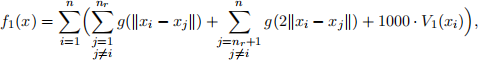 (4)
(4)
for x = (x1 , x2 , . . . , xn) e R2n, and where f2 is defined identically, except with V1 replaced by V2 .
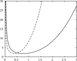
Figure 1: Plots of the functions g(r), shown by a solid line, and g(2r), shown by a dashed line.
(a) What is the formula for the gradient lf1 (x)? Hint: Consider the formula for each term ∂f1 (x)/∂(xi)e separately, where v = 1, 2 and i = 1, 2, . . . , n. You can verify that your formula is correct by comparing the value to a corresponding finite difference approximation.
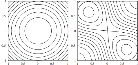
Figure 2: Contour plots of the functions V1(x) and V2(x), produced by the command contour.
(b) For n = 1, f1 is convex. Why is f2 not convex for n = 1? Why are neither f1 nor
f2 convex for n > 1?
(c) What is the cost of evaluating f1 (x) or f2 (x), in big-O notation? What is the cost of evaluating lf1 (x) or lf2 (x)?
2. Consider the optimization problems
 (5)
(5)
and
 (6)
(6)
Implement the Polak-Ribi`ere (PR) method in MATLAB, using the provided line search function linesearch .m, to solve problem (5). Set the Wolfe condition parameters to c1 = 0.0001 and c2 = 0.2, and use α 1 = 0.0001 as the initial step length and αmax = 1 as the maximum step length. Iterate for maxiter = 100 iterations, or until the first-order optimality condition |lf(x)| < tol is attained, where tol = 10_2 . Keep track of the number of times f(x) or lf(x) are computed. Use the provided function printiter .m to print, at each iteration, the iteration number, the number of function evaluations so far, the value of f(xk), the step size αk, and the optimality condition |lf(xk)|, printing the header every 20 iterations. Hint: Implement f(x) and lf(x) as functions f and df, so that x and df(x) are 2 x n- matrices. Then, provide the wrapper functions h=@(x) f(reshape(x,2,n)) and dh=@(x) reshape(df(reshape(x,2,n)),2*n,1) to your algorithm.
(a) Solve (5) for n = 50 and nr = 20. Set x0 e R2n using the command x0=rand(2,n) - [0 .5;0 .5], executing the command rng(112) before the rand function is called in order to set the seed of the pseudo-random number generator. Plot the solution returned by your algorithm on top of the contour plot shown in Figure 2, denoting
the red particles by red x’s and the blue particles by blue x’s, and setting both x- and y-limits to [_0.8, 0.8]. Show the last 5 lines of the output of printiter .m.
(b) Repeat these same steps, but for nr = 35. What do you see?
(c) Try part (a) again, this time setting c1 = 0.1 while leaving c2 = 0.2 unchanged. What do you observe? Try it once more, setting c2 = 0.001 while leaving c1 = 0.0001 unchanged. What do you observe? How sensitive is the algorithm to c1 and c2 ?
(d) Repeat part (a), except this time, solve (6).
(e) Implement the Fletch-Reeves (FR) method. Repeat part (d), setting maxiter =
400. You do not need to show the solution plots or the output of printiter .m. Plot |lf(xk)| using the semilogy command for both PR and FR on the same plot, making sure to use the same initial guess x0 for both methods. What do you see?
(f) One resetting strategy for nonlinear conjugate gradient methods is to reset the
iteration whenever two consecutive gradients are far from orthogonal, since this indicates that f(x) does not resemble a quadratic function. Try part (d) again, with maxiter = 400, but this time, set βk+1 = 0 whenever
 (7)
(7)
where ν = 0.1. You do not need to show the solution plots or the output of printiter .m. Plot |lf(xk)| using the semilogy command for both PR with this restarting strategy, and PR without it, on the same plot. Do you see much benefit?
(g) Repeat part (e), but this time, compare PR, FR-PR, and PR+. What do you see?
(h) Why do your implementations of these nonlinear conjugate gradient methods only
converge linearly? What modification(s) are required to produce n-step quadratic convergence?
3. Implement the BFGS method in MATLAB, using the provided line search function linesearch .m, to solve problem (6). Store and update the matrix Hk naively, as a dense matrix. Set the Wolfe condition parameters to c1 = 0.0001 and c2 = 0.9, and use α 1 = 1 and αmax = 10. Set maxiter = 500 and tol = 10_2 , and use printiter .m as described in problem 2.
(a) Repeat problem 2(a), omitting the solution plot, setting H0 = I. Plot |lf(xk)|
using the semilogy command. At which iteration does the method begin to converge superlinearly?
(b) If H0 not chosen to be similar to l2 f(x0 )_1 , then the initial step α 1 = 1 can be
far too long, and must be reduced at the cost of many function evaluations. One way to make the size of Hk to be similar to the size of l2 f(xk)_1 early on is to set H0 = I, and then set
 (8)
(8)
at the first iteration (see ?6.1 in Nocedal and Wright). Repeat part (a), with this change to H1 . Plot |lf (xk)| using the semilogy command, for BFGS both with and without this choice of H1, on the same plot. What do you see?
(c) Implement the DFP method, with the same modification to H1 as in part (b). Plot |lf (xk)| using the semilogy command for both BFGS and DFP (both with modified H1) on the same plot. What do you see?
4. Exercise 6.9.
