EEE404/591 Real Time DSP Project 1

I.           Objectives

The objective of this project is to apply simple real time image enhancement techniques to live video stream captured from a webcam. Upon completion, students will be familiar with

•    the process of capturing image frames from webcam using MATLAB, sending them through   serial port to board to process, and receiving the processed frames in MATLAB to display and

compare

•    coding image processing algorithms including quantization, thresholding, gray level transformations and histogram equalization

II.          Hardware Setup

Set up the following hardware :

•    STM32F407G-DISC1 kit: When you are ready to upload code to your board, connect USB Type-A end of the cable to your computer’s USB port, connect the Mini-B end of the cable to the board. The PWR red LED will turn on.

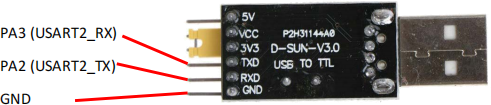
•   To establish serial communication between your computer and board for video streaming, make the following connections between the STM32F407 board header pins PA2, PA3, GND, and the   serial/USB converter:

•    Webcam: a webcam is needed to capture video frames for streaming

III.         Software Setup

MATLAB is needed to capture video frames, establish serial communication between computer and board, send and receive video frames, and plot them for comparison.

You need to install the MATLAB Support Package for USB Webcams at https://www.mathworks.com/matlabcentral/fileexchange/45182-matlab-support-package-for-usb- webcams

If you see error message stating “USB device not recognized” when you plug in the serial/USB converter, you need to install the CH340 driver. Instructions can be found at  https://learn.sparkfun.com/tutorials/how-to-install-ch340-drivers/all.

IV.        Code

Download the following code from Canvas:

•    main_testing.c

•    main.c

•    capture_frames_connect_serial_plot_compare.m

V.         References

The following documents are posted on Canvas.

•    STM32CubeIDE User Guide

•    STM32F407 Discovery Board User Manual

•    STM32F4 Drivers

VI.        Tasks

Gray scale 8-bit per pixel video frames will be sent to the board. The board will process the images          implementing the following algorithms and send back the processed images. The original and processed images will then be displayed for comparison. It is recommended that you complete Task 1, 2, 3 in week 1 and Task 4 in week 2.

1.    Thresholding

Thresholding, also known as segmentation, aims to divide the image into a foreground and a background. It can also be used to divide the image into a region of interest and background. Three methods will be used:

•    Global thresholding

•    Band thresholding

•    Semi thresholding

1)    Global thresholding:

This is the simplest segmentation algorithm. An image is reduced to two levels using the following equation:

f(x, y) =

if p(x, y) ≥ T

if p(x, y) < T

As shown in the equation, all pixels less than the threshold T are set to black (intensity value=0) and all pixels equal to or above the threshold are set to white (intensity value=255). To choose a suitable threshold you may want to plot the histogram of your scene and try to deduce the value. Usually thresholds are chosen at the valleys of the histogram.

2)    Band thresholding

Most of the time when the histogram cannot be clearly separated into two regions, one may want to use what is called “Band Thresholding” technique, where:

f(x, y) =

if p(x, y) e D

otheTwise

Band thresholding will segment an image into regions of pixels with gray levels from a set D and into background. The set D chooses the “region of interest” . This method can be used to generate a mask corresponding to the region of interest. For this project, the following equation will be implemented:

f(x, y) =

if T1  ≤ p(x, y) ≤ T2

otherwise

3)    Semi thresholding

Semi thresholding assigns a grayscale value 0 (black) to the background. For a given threshold T, the equation is:

f(x, y) = {  p(x, y)

if p(x, y) ≥ T

if p(x, y) < T

For the above thresholding algorithms, you need to perform the following tasks:

•    Global thresholding (write C function, hybrid assembly function provided as an example)

•    Band thresholding (write C function, GRAD STUDENTS ONLY write hybrid assembly function)

•    Semi thresholding (write C function, write hybrid assembly function)

Based on your image’s histogram, choose appropriate thresholds to separate pixels into foreground and background in order to highlight different features. Write down your thresholds and include a screenshot of the MATLAB plot for each scenario.

2.    Gray level quantization

Often, grayscale images are represented using 8 bits for each pixel resulting in 256 levels. The human  visual system can only differentiate up to 100 levels at most. 256 levels are used because artifacts and noise can be hidden thus exploiting the limitations of our visual system. Another reason is that most processors support 8-bit arithmetic.

Quantization aims to achieve a reduction in the memory or bitrate requirements by reducing the precision. For example, if 4 bits are used to represent a pixel instead of 8, two pixels can be represented in a byte thus reducing memory requirements. However, reduction in precision can affect perceived image quality. We will observe the effect by reducing the number of levels from 256 to 128, 64, 32 and  16 and observing the resulting change in image quality. To perform quantization, for example, from 256 to 128, divide each pixel by two or shift to the right by one.

The board will quantize the images and send the quantized images back to your computer. MATLAB is    used to reconstruct the quantized images and observe the change in image quality if there is any. For example, if the number of gray scale levels are reduced from 256 to 32 levels, the images are quantized by dividing each pixel by 8, i.e., right shifting by 3. The resulting quantized pixels are in the range 0-31. If this is directly plotted in MATLAB, one will not be able to see the effect of the quantization error. Moreover, the image intensity is reduced. You need to modify the MATLAB script to reconstruct the image by multiplying each pixel by 8 (i.e., left shifting by 3) before displaying it.

For the above gray level quantization algorithm, you need to perform the following tasks:

•    Gray level quantization (write C function, write hybrid assembly function)

•    Modify provided MATLAB script to reconstruct quantized image for display

Quantize the images from 256 levels to 128, 64, 32 and 16 levels. Record your observations and answer the following questions in the table below. Include a screenshot of the MATLAB plot for each scenario.

1)    Do you observe any degradation in image quality due to the quantization?

2)    Do you observe any missing values in the histogram of the reconstructed image at locations where there were values in the original histogram? Why?

3.    Gray level transformations

In this part, you will implement some of the gray level transformations such as negative, brightness and contrast transformations to enhance the input image.

An image processing system that looks at every input pixel gray level and generates a corresponding output  gray  level  according  to  a  fixed  gray  level  mapping  function  implements  a  basic  gray  level transformation. You might think of this transformation as an analytic function or a mapping performed through a discrete table. The figures below represent three gray level transformation algorithms.

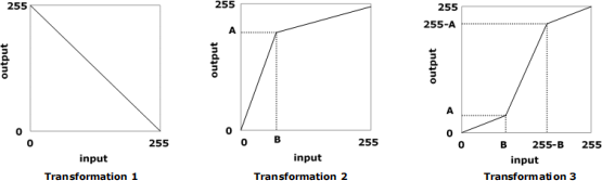
The transformation equations can be derived from the graphs, and are provided to you for your convenience:

Transformation 1:

Transformation 2:

f(x, y) =  (2(2)5(5)5(5)  B(A) − B) + A

if 0 ≤ p(x, y) ≤ B

if B ≤ p(x, y) ≤ 255

p(x, y)                      () (p(x, y) − B) + A

 (p(x, y) − (255 − B)) + (255 − A)

if 0 ≤ p(x, y) ≤ B

if B ≤ p(x, y) ≤ 255 − B

if 255 − B ≤ p(x, y) ≤ 255

For the above gray level transformation algorithms, you need to perform the following tasks:

•    Transformation 1 (write C function, write hybrid assembly function)

•    Transformation 2 (write C function, GRAD STUDENTS ONLY write hybrid assembly)

•    Transformation 3 (write C function, write hybrid assembly function for extra credit of 10 points)

Note:

1)   While implementing the transformations in C, make sure you perform all divisions in float. You    can do this by casting the dividend and the divisor to float. For example, if you are calculating y = AX/B, and A=50 and B=75, A/B=0 if integer division is performed. Then all values of y computed   using this equation would be zero. This would result in black spots in the output image. To solve this problem, you can perform (float) (A*x)/ ((float) (B)) to get a floating-point result. If x=50,        A=50 and B=75, this would result in 33.333. This result can then be written back into y by casting it back into the required type. Casting back to integer would result in 33 being written into y.

2)   When implementing the transformations in assembly, use MUL and UDIV instructions for         multiplications and divisions. Make sure you do MUL first before you UDIV, otherwise you will get zero like the example described above.

For Transformation 2 and Transformation 3, choose different values of A and B and perform at least 3

cases:

1)   A less than B

2)   A greater than B

3)   A equal to B

For Transformation 2, while choosing A and B, make sure that A < (255-A) and B< (255-B).  What          happens if A=B in Transformation 2 or Transformation 3? Identify the effect introduced by each           transformation and document your results in the following table. Include a screenshot of the MATLAB plot for each scenario.

4.    Histogram equalization

If 8 bits are used to represent a pixel, that pixel can have any value between 0 (black) and 28-1= 255 (white). Thus, the total dynamic range of the grayscale levels is 256. Often, images tend not to make use of the total dynamic range available to them. Although 256 gray levels can theoretically be used to represent the image samples, the entire range is rarely utilized. The effect of dynamic range misuse is a  poor image contrast. To remedy this problem, it is possible to use the histogram to generate a special     gray level mapping suited for a particular image at hand. This process is called histogram equalization.

Recall the steps of histogram equalization from lecture (N = number of pixels in the image, L = number of gray scale levels = 256):

1)    Compute image histogram: ℎist(i), i  =  0, … , L − 1

2)    Normalize histogram: normalize amplitudes so that the sum of all values is equal to one and you have a pdf: pdf(i) =  , i  =  0, … , L − 1

3)   Compute a cdf(i) = ∑ k(i)=0 pdf(k) and mappingtable[i] = int[(L − 1)cdf(i)] =

int l] , i  =  0, … , L − 1. Instead of using the rounding operation discussed in the lecture, we simply cast the result to an integer.

4)    Map pixels in the image from old gray scale level to new level based on the mapping table.

The pseudo code for the histogram equalization is shown below:

Initializing_Phase

Assume original image is stored in image_org and resultant image in image_equ

Let N be the number of pixels for each frame

Let L = 256 (number of grayscale levels)

Define buffers hist[L], mapped_levels[L]

Initialize elements of hist to 0

calculate_histogram (step 1)

For i = 1 → N

Temp = current pixel value

Increment hist[temp]    // counting the number of occurrences of  each level

End For

map_levels (on the fly) (step 2 and 3)

For i= 1 → L

Update sum = accumulated histogram count

mapped_levels[i] = (int)(L-1)*sum/N

End For

transform_image (step 4)

For i = 1 → N

img_equ[i] = mapped_levels[img_org[i]]

End For

Note: When implementing the “map_levels” function above in assembly, use MUL and UDIV instructions for multiplications and divisions. Make sure you do MUL first before you UDIV, i.e., do (L −

1) ∑k(i)=0 ℎist(k) first, then , if you do  first, then (L − 1) , you will always get zero.

You need to perform the following tasks for the algorithm:

•    calculate_histogram (write C function, write hybrid assembly function)

•    map_levels (write C function, write hybrid assembly function)

•    transform_image (write C function, write hybrid assembly function)

Fill in the following table and comment on the difference you observe between the original and the processed images, and include a screenshot of the MATLAB plot.

VII.       Deliverables

Start your lab report by including the lab title and your name at the top.

Include in your lab report the followings. Submit your lab report as a single PDF file to Canvas.

1.   Table (4) : the filled-out tables from the four tasks above.

2.    Screenshot (4):

Show screenshots for the following functions, one for each function (use test vector

trmt_data[BUFFER_SIZE] = {122, 155, 80, 254, 7, 40, 240, 50} in main_testing.c):

void semi_thresholding_hybrid(uint8_t *x, uint32_t size, uint8_t threshold);

void gray_level_quantization_hybrid(uint8_t *x, uint32_t size, uint8_t shift_factor); void gray_level_transformation1_hybrid(uint8_t *x, uint32_t size);

Show one screenshot for the three histogram equalization functions altogether (use test vector trmt_data[BUFFER_SIZE] = {1, 1, 3, 5, 6, 7, 7, 7} in main.testing.c):

void calculate_histogram_hybrid(uint8_t *x, uint32_t *hist, uint32_t size);  void map_levels_hybrid(uint32_t *hist, uint8_t *mapping_table, uint32_t size, uint16_t levels);

void transform_image_hybrid(uint8_t *x, uint8_t *mapping_table, uint32_t size);

Show screenshot for the following function for extra credit:

void gray_level_transformation3_hybrid(uint8_t *x, uint32_t size, uint8_t a0, uint8_t b0);  (10 pts)

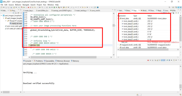
The screenshot should display the image processing function(s) and the program stopping at breakpoint “while (1)” on the left, and the value of the trmt_data array on the right (see below).

3.    Code:

Include the NEW code you added or modified in the MATLAB script for image reconstruction after gray level quantization.

Include the C and hybrid assembly functions required in the four tasks above.

// segmentation/thresholding functions

void global_thresholding_c(uint8_t *x, uint32_t size, uint8_t threshold);

void band_thresholding_c(uint8_t *x, uint32_t size, uint8_t threshold1, uint8_t threshold2);

void semi_thresholding_c(uint8_t *x, uint32_t size, uint8_t threshold);     void semi_thresholding_hybrid(uint8_t *x, uint32_t size, uint8_t threshold);

// gray level quantization functions

void gray_level_quantization_c(uint8_t *x, uint32_t size, uint8_t shift_factor);     void gray_level_quantization_hybrid(uint8_t *x, uint32_t size, uint8_t shift_factor);

// gray level transformation functions

void gray_level_transformation1_c(uint8_t *x, uint32_t size);

void gray_level_transformation1_hybrid(uint8_t *x, uint32_t size);

void gray_level_transformation2_c(uint8_t *x, uint32_t size, uint8_t a0, uint8_t b0); void gray_level_transformation3_c(uint8_t *x, uint32_t size, uint8_t a0, uint8_t b0);

// histogram equalization functions

void calculate_histogram_c(uint8_t *x, uint32_t *hist, uint32_t size);     void calculate_histogram_hybrid(uint8_t *x, uint32_t *hist, uint32_t size);

void map_levels_c(uint32_t *hist, uint8_t *mapping_table, uint32_t size, uint16_t levels);

void map_levels_hybrid(uint32_t *hist, uint8_t *mapping_table, uint32_t size, uint16_t levels);