关键词 > STA437H1S/2005H1S
Assignment #1 STA437H1S/2005H1S
发布时间:2023-02-21
Hello, dear friend, you can consult us at any time if you have any questions, add WeChat: daixieit
Assignment #1 STA437H1S/2005H1S
due Friday February 3, 2023
Instructions: Solutions to problems 1–4 are to be submitted on Quercus (PDF files only).
1. Suppose that u = (X1 , . . . , X5 )T ~ N5 (μ, C) where
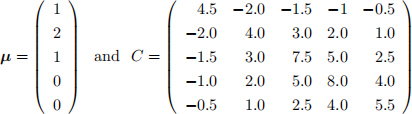
(a) What are the marginal distributions of X1 , . . . , X5 ?
(b) What is the conditional distribution of (X1, X2 ) given X3 = 2, X4 = 3 and X5 = _1? (You should use R or some other software to compute whatever matrix inverses you need.)
(c) Using the inverse of C, give the graph structure of the dependence in u . (Again use R to compute C←1 but note that the numerical computation is subject to roundoff error!)
2. The file marks .txt on Quercus contains the exam marks data considered in lecture. In that analysis, we assumed that the data came from a multivariate Normal distribution. The data can be read into R as follows:
> exam <- scan("marks .txt",what=list(0,0,0,0,0))
> mec <- exam[[1]]
> vec <- exam[[2]]
> alg <- exam[[3]]
> ana <- exam[[4]]
> sta <- exam[[5]]
(a) Look at Normal quantile-quantile plots of the 5 variables separately using qqnorm. You can judge the “goodness-of-fit” using the Shapiro-Wilk test, which can be implemented in R using shapiro .test. Comment on the results.
(b) Use the function qqmultinorm (which is in the file qqmultinorm .txt on Quercus) to assess the multivariate normality of the data. The following R code will look at 100 Normal quantile-quantile plots of 100 randomly chosen projections and compute p-values for the Shapiro-Wilk test for each projection:
> r <- qqmultinorm(cbind(mec,vec,alg,ana,sta),nproj=100,plot .edf=T)
The plot produced will be the empirical distribution function of the 100 p-values compared to the distribution function of a uniform distribution on [0 , 1]. Based on this plot, do the data seem to be (at least approximately) multivariate Normal?
(c) The other approach to testing multivariate normality given in lecture is to compare the empirical distribution of the Mahalanobis distances {(ai _ ![]() )T S ←1(ai _
)T S ←1(ai _ ![]() ) : i = 1, . . . , n} to a χ2 (5) distri- bution. If the data are contained in an n × p matrix, the Mahalonobis distances can be computed in R as follows:
) : i = 1, . . . , n} to a χ2 (5) distri- bution. If the data are contained in an n × p matrix, the Mahalonobis distances can be computed in R as follows:
> mdist <- mahalanobis(x,colMeans(x),var(x))
Does this plot confirm your conclusion from part (b)?
3. The file crabs .txt on Quercus contains data on two species of rock crabs, which are distinguished by their colour (blue or orange); the columns of the file are species (B or O), sex (M or F), index (1-50 within each species-sex combination), width of the frontal lip (LP), the rear width of the shell (RW), length along the midline of the shell (CL), the maximum width of the shell (CW), and the body depth (BD). Ultimately, we would like to use the latter 5 variables to classify the species and sex of a crab but at this stage, we will simply look at the structure of the data to see which variables might be useful in classifying the species and sex of a rock crab.
The data can ne read into R using the following code:
> x <- scan("crabs .txt",skip=1,what=list("c","c",0,0,0,0,0,0))
> colour <- ifelse(x[[1]]=="B","blue","orange")
> sex <- x[[2]]
> FL <- x[[4]]
> RW <- x[[5]]
> CL <- x[[6]]
> CW <- x[[7]]
> BD <- x[[8]]
Use the following code to look at pairwise scatterplots of the 5 variables:
> pairs(cbind(FL,RW,CL,CW,BD),pch=sex,col=colour)
The males and females are indicated on the plots by M and F respectively with the two species being indicated by the colour of the points.
(a) Which pairwise scatterplots are particularly effective for “separating” the two species? (b) Which pairwise scatterplots are effective for “separating” the two sexes?
4. In class, we stated that we can assess whether multivariate data can be modeled by a multivariate Normal distribution by checking the normality of a collection of one dimensional projections (for example, by using normal quantile-quantile plots). When p is very large, this procedure breaks down – almost every one dimensional projection appears to be Normal.
(a) Consider n=100 observations of a 1000-variate distribution whose components are independent exponential random variables with mean 1; the joint density of this distribution is
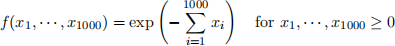
We can simulate the 100 observations in R as follows:
> x <- matrix(rgamma(100000,1),ncol=1000)
Now use the function qqmultinorm (available on Quercus) to look at normal quantile-quantile plots of 20 one dimensional projections:
> r <- qqmultinorm(x,nproj=20,plot .qq=T,plot .edf=T)
How do these quantile-quantile plots compare to the quantile-quantile plots of each variable (for example, qqnorm(x[,1]))?
(b) Can you explain this phenomenon? (Hint: What is the approximate distribution of aT u = j(p)=1 ajXj when p is large if max1←j←p aj(2)/aT a is small?)
