PSTAT 174/274: Homework # 4

Hello, dear friend, you can consult us at any time if you have any questions, add WeChat: daixieit

PSTAT 174/274: Homework # 4.

1. (both 174 & 274 attempt) Topic: Autocorrelation Functions

Note:  {Zt} ∼ WN (0, σZ(2)) denotes white noise.

Question: Bellow, you are given the following graphs of autocorrelation functions for three separate data sets, each with n observations.  The dotted lines in each graph correspond to 95% confidence intervals. Determine which of the above data sets exhibit statistically significant autocorrelations. Explain how you came to this conclusion.

A. I only;   B. II only;   C. III only;   D. I, II and III;   E. The answer is not given by (A), (B), (C), or (D).

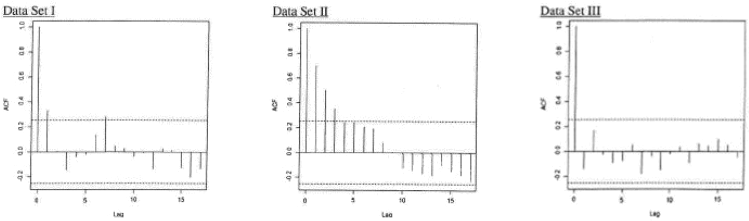
Figure 1:  Autocorrelation functions.  Left plot - Data set I, Middle plot - Data Set II, Right plot - Data Set III.

2. (both 174 & 274 attempt) Topic: stationarity and invertibility

For the following two time series models, check stationarity and invertibility. Fully justify your answer.

i Xt = Zt − Zt − 1 − Zt −2 .

ii Xt = Xt − 1 + Xt −2 + Zt .

3. (both 174 & 274 attempt) Topic: Autocorrelation Functions

Questions:

a For a MA(3) process with coefficients θ 1 = 2, θ2 = 0.5, and θ3 = −0.1,

i write the mathematical equation for MA(3) model with these coefficients, and    ii calculate the autocorrelation function at lags 1, 2, 3, 4: ρ(1), ρ(2), ρ(3) and ρ(4).

b For an AR(1) process with coefficient ϕ 1 = −0.5,

i write the mathematical equation for AR(1) model with these coefficients, and    ii calculate the autocorrelation function at lags 1, 2, 3, 4: ρ(1), ρ(2), ρ(3) and ρ(4).

4. (both 174 & 274 attempt) Topic: Time Series Linear Regression with ARIMA errors

You will undertake a time series regression where the response is a measure of the thickness of deposits of sand and silt (varve) left by spring melting of glaciers about 11,800 years ago.  The data are annual estimates of varve thickness at a location in Massachusetts for 455 years beginning 11,834 years ago.

Consider the data set for the response in the astsa package in R: astsa::varve data and undertake the following analysis.

•  Create a plot of the response as a time series plot and create some of the seasonal plots we have explored in class - what structure does this time series have?

• For the response time series - what do you observe?  (should you consider a Box-Cox transform?)

•  Observe that for the response time series there is a curve linear pattern (trend) over time. Suggest a suitable trend function and fit this regression of yt  vs trend function of time f (t) and additive error et .

• Plot the ACVF and ACF of the residuals from your selected model.

• What do you see?

• Now consider the model as having AR(1) errors and apply the Cochrane-Orcutt procedure.  Write down the formula for the adjusted estimator and explain why such an adjustment may be needed.