Week 10 Tutorial Sheet (Solutions)

Week 10 Tutorial Sheet

(Solutions)

Useful advice: The following solutions pertain to the theoretical problems given in the tutorial classes. You are strongly advised to attempt the problems thoroughly before looking at these solutions. Simply reading the solu-tions without thinking about the problems will rob you of the practice required to be able to solve complicated problems on your own. You will perform poorly on the exam if you simply attempt to memorise solutions to the tutorial problems. Thinking about a problem, even if you do not solve it will greatly increase your understanding of the underlying concepts. Solutions are typically not provided for Python implementation questions. In some cases, psuedocode may be provided where it illustrates a particular useful concept.

Assessed Preparation

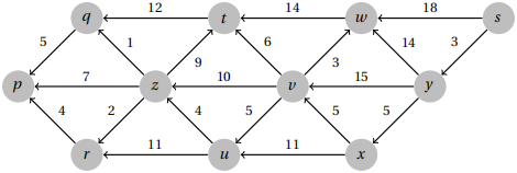
Problem 1.  Use Dijkstra’s algorithm to determine the shortest paths from vertex s to all other vertices in this graph. You should clearly indicate the order in which the vertices are visited by the algorithm, the resulting distances, and the shortest path tree produced.

Solution

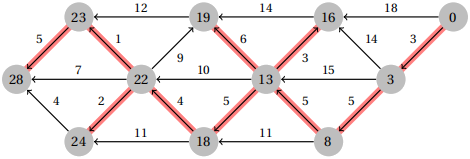
Vertices are visited in the order:

s, y, x, v, w, u, t, z, q, r, p

The shortest path tree, with vertices labelled by their distances is shown

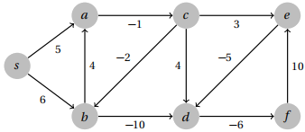
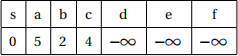
Problem 2.  Use Bellman-Ford to determine the shortest paths from vertex s to all other vertices in this graph. Afterwards, indicate to which vertices s has a well defined shortest path, and which do not by indicating the distance as −∞. Draw the resulting shortest path tree containing the vertices with well defined shortest paths. For consistency, you should relax the edges in the following order: s → a, s → b, a → c, b → a, b → d, c → b, c → d, c → e, d → f, e → d and f → e .

Solution

The distances at each iteration are shown below. If you followed the order specified, you should have the same distances. Relaxing the edges in a different order may lead to a different table, but the end distances should be the same (except for the vertices reachable via negative cycles).

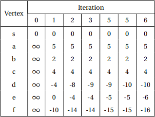
Since another round of relaxation would decrease the distance of vertex d , it must be reachable via a negative cycle. All of the vertices reachable from d therefore have undefined distance estimates. The final distances are therefore

The shortest path tree is shown below

Tutorial Problems

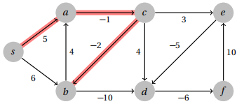
Problem 3.  Give an example of a graph with negative weights on which Dijkstra’s algorithm produces the wrong answer.

Solution

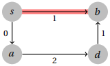
Many graphs are possible. The key is to force Dijkstra’s to take a wrong path by hiding a beneficial negative weight edge behind a higher weight edge. The following example does this.

In this case, Dijkstra will take the highlighted path, which is not a shortest path.

Problem 4.  Consider the following algorithm for single-source shortest paths on a graph with negative weights:

• Find the minimum weight edge in the graph, say it has weight w

• Subtract w from the weight of every edge in the graph. The graph now has no negative weights

• Run Dijkstra’s algorithm on the modified graph

• Add w back to the weight of the edges and compute the lengths of the resulting shortest paths

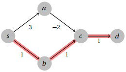
Prove by giving a counterexample that this algorithm is incorrect.

Solution

The problem with this algorithm is that it changes the length of paths with more edges a larger amount than it changes the lengths of paths with fewer edges, since it adds a constant amount to every edge weight. A good graph to break this would therefore be one where a shortest path has more edges than an alternative.

In this case, the shortest path from s to b is s → a → d → b with length −12. If we subtract −5 from every edge weight in the graph, then it becomes the following, where the shortest path is now s → b , so we get the wrong answer.

Problem 5.  Suppose that we wish to solve the single-source shortest path problem for graphs with nonnegative bounded edge weights, i.e. we have w(u, v) ≤ c for some constant c . Explain how we can modify Dijkstra’s algorithm to run in O(V + E) time in this case. [Hint: Improve the priority queue]

Solution

The part of Dijkstra’s algorithm that adds the log factor is the priority queue, so let’s try to improve that. Given that the edge weights are bounded above by c , and a shortest path can contain at most V −1 edges, the largest distance estimate that we can ever have is less than c V . Also observe that since we remove vertices from the priority queue in distance order, the minimum element in the priority queue never decreases. We can use these two facts to make a faster priority queue for Dijkstra’s.

Let’s just store an array of size c V , where at each entry, we store a linked list of vertices who have that distance estimate. Adding an element to this priority queue takes O(1) since we can simply append to the corresponding linked list. Updating a distance estimate can also be achieved in O(1) since we can remove an element from a linked list in O(1) and append it to a different one. Since the minimum distance for entries obtained from priority queue never decreases, we can simply move through the priority queue, starting at distance zero and moving onto the next distance when there are no vertices left to process at the current distance. We never move back to a previous distance.

All updates to the priority queue take O(1). Finding the minimum element in the priority queue could take up to O(V), but note that since we never go backwards, the total time complexity of all find minimum operations will be O(V), since scanning all of the distances takes O(c V) = O(V) since c is a constant. The total time complexity of Dijkstra’s using this priority queue will therefore be O(V + E).

Problem 6.  Describe an algorithm that given a graph G determines whether or not G contains a negative cycle. Your algorithm should run in O(V E) time.

Solution

Remember that the Bellman-Ford algorithm can detect whether there is a negative cycle that is reach-able from the source vertex. The obvious tempting solution is to just run Bellman-Ford from every pos-sible source vertex and see whether a negative cycle is detected. This would be very slow though, taking O(V² E) time. Instead, we would rather run just one Bellman-Ford, but how can we be sure that we can definitely reach the negative cycle if one exists? The easiest way to ensure this is to simply add a new vertex to the graph, and add an edge from that vertex to every other vertex in the graph. Running Bellman-Ford on this vertex will then definitely visit every vertex, and hence will definitely detect a negative cycle if one is present. Since we only need to run Bellman-Ford once, this algorithm takes O(V E ) time.

Problem 7.  Improve the Floyd-Warshall algorithm so that you can also reconstruct the shortest paths in addition to the distances. Your improvement should not worsen the time complexity of Floyd-Warshall, and you should be able to reconstruct a path of length k in O(k) time.

Solution

There are many approaches to make this work.

Solution 1: Track the intermediate vertex

The simplest way to keep track of the path information is to record, for each pair of vertices u, v, which intermediate vertex was optimal for going between them. This can be tracked during the algorithm like so.

1: function FLOYD_WARSHALL(G = (V, E))

2:     Set dist[1..n][1..n] = ∞

3:     Set dist[v][v] = 0 for all vertices v

4:     Set dist[u][v] = w(u,v) for all edges e = (u,v) in E

5:     Set mid[1..n][1..n] = null // mid[u][v] = optimal intermediate vertex

6:     for each vertex k = 1 to n do

7:         for each vertex u = 1 to n do

8:             for each vertex v = 1 to n do

9:                 if dist[u][k] + dist[k][v] < dist[u][v] then

10:                     dist[u][v] = dist[u][k] + dist[k][v]

11:                     mid[u][v] = k

12:                 end if

13:             end for

14:         end for

15:     end for

16:     return dist[1..n][1..n], mid[1..n][1..n]

17: end function

To reconstruct the path, we then need to do a sort of divide-and-conquer style path reconstruction.

1: function GET_PATH(u, v)

2:     if mid[u][v] = null then

3:         return [u, v]

4:     else

5:         left = GET_PATH(u, mid[u][v])

6:         right = GET_PATH(mid[u][v], v)

7:         return left.pop_back() + right // Remove the duplicate from the middle

8:     end if

9: end function

Solution 2: Track the successor

Another slightly cleaner solution is to remember for each pair u, v , what is the first vertex on a shortest path from u to v . To maintain this, if we update the pair u, v and decide that vertex k is the new best intermediate vertex, then the first vertex on a shortest path from u to v is just the first vertex on a shortest path from u to k. We can implement this as follows.

1: function FLOYD_WARSHALL(G = (V, E))

2:     Set dist[1..n][1..n] = ∞

3:     Set dist[v][v] = 0 for all vertices v

4:     Set dist[u][v] = w(u,v) for all edges e = (u,v) in E

5:     Set succ[1..n][1..n] = null // succ[u][v] = successor of u on shortest path to v

6:     Set succ[u][v] = v for all edges e = (u,v) in E

7:     for each vertex k = 1 to n do

8:         for each vertex u = 1 to n do

9:             for each vertex v = 1 to n do

10:                 if dist[u][k] + dist[k][v] < dist[u][v] then

11:                     dist[u][v] = dist[u][k] + dist[k][v]

12:                     succ[u][v] = succ[u][k]

13:                 end if

14:             end for

15:         end for

16:     end for

17:     return dist[1..n][1..n], succ[1..n][1..n]

18: end function

Reconstructing the paths is now easier as we do not need any fancy recursion.

1: function GET_PATH(u, v)

2:     Set path = [u]

3:     while u v do

4:         u = succ[u][v]

5:         path.append(u)

6:     end while

7: end function

In both cases, we add only a constant amount of overhead to the algorithm so we do not worsen the complexity. We can also reconstruct paths of length k in O(k) time in both cases.

Problem 8.  Consider the problem of planning a cross-country road trip. You have a map of Australia consisting of the locations of towns, each of which has a petrol station, with the corresponding petrol prices (which may be different at each town). You are currently at a particular town s and would like to travel to town t . Your car has a fuel capacity of C litres, and for each road on the map, you know the amount of petrol it will take to travel along it. Your tank can only contain non-negative integer amounts of petrol, and all roads cost an integer amount of petrol to travel along. You can not travel along a road if you do not have enough petrol to make it all the way. You may refuel at any petrol station whether your tank is empty or not (but only to integer values), and you are not required to fill your tank. Assuming that your tank is initially empty, describe an algorithm for determining the cheapest way to travel to city t . [Hint: You should model the problem as a shortest path problem and use Dijkstra’s algorithm.]

Solution

Our first thought might be to weight the edges of the graph by how much petrol they use and then run Dijkstra’s algorithm, but this will miss quite a few things. Remember that we need to take into account:

• The cost of petrol at various towns

• We can fuel up partially at any town, and leave the town with any amount of petrol

• We might not be able to make it across a road without running out

In order to account for these things, we create a new graph that encapsulates more information than just our location on the vertices. Suppose that there are n towns Let’s make a graph that contains (C + 1)n vertices, one for each town for each possible amount of petrol that we could possible have. That is, each town has (C + 1) different vertices, one for when we are in that town with no petrol, one for when we are there with 1 litre, 2 litres and so on. Let’s the use the notation 〈u, c〉 to denote the vertex corresponding to town u where we have c litres of petrol currently in the tank.

If a road from town u to town v takes x litres of petrol to travel, then for each of the vertices 〈u, c〉 corre-sponding to town u with c ≥ x , we create an edge to the corresponding vertex 〈v, c − x〉 of town v . For example, if x = 5, then we create an edge from 〈u, 10〉to 〈v, 5〉, and from 〈u, 9〉to 〈v, 4〉, from 〈u, 8〉to 〈v, 3〉, and so on. Importantly, these edges have weight zero, since we are going to use edge weights to model the cost of purchasing fuel.

To account for buying new fuel, suppose we are currently in the town u whose petrol price is p. Then we should add an edge from every vertex 〈u, c〉 with c < C to the vertex 〈u, c + 1〉 with weight p. Note that we could have added edges from 〈u, c〉 to 〈u, c + 2〉 with weight 2p and so on, but this would just make the graph unnecessarily denser and hence make the algorithm slower for no reason, so it is best to simply add edges that add 1 litre of petrol at a time.

We can then run Dijkstra from the vertex 〈s, 0〉to find the shortest path to 〈t , 0〉, which will be the cheapest way to make it from s to t .

Supplementary Problems

Problem 9.  Implement Dijkstra’s algorithm and test your code’s correctness by solving the following Codeforces problem: http://codeforces.com/problemset/problem/20/C.

Problem 10.  Implement Bellman-Ford and test your code’s correctness by solving the following problem on UVA Online Judge: https://uva.onlinejudge.org/index.php?option=onlinejudge&page=show_problem&problem=499.

Problem 11.  Consider a buggy implementation of Dijkstra’s algorithm in which the distance estimate to a vertex is only updated the first time the vertex is discovered, and not in any subsequent relaxations. Give a graph on which this bug will cause the algorithm to not produce the correct answer.

Solution

To break such a bug, we need a vertex whose initial distance estimate is very high, but should be subse-quently lowered by a better path found later. The following graph will cause this problem.

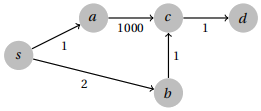
The distance estimate to c will get locked at 1001, even though it should be updated to 3, and hence the distances to c and d will be wrong.

Problem 12.  Given a graph that contains a negative weight cycle, give an algorithm to determine the vertices of one such cycle. Your algorithm should run in O(V E ) time.

Solution

Recall from Problem 6 that we can use Bellman-Ford to detect the presence of a negative cycle by adding a new source vertex that connects to all others. Let’s start by doing this. Remember that when Bellman-Ford terminates, the predecessors will all form a shortest path tree, except for the vertices reachable from a negative cycle. These predecessors may not form a tree, but may actually form cycles since they will point to the vertices that caused them to relax most recently. To guarantee that the predecessors form a cycle, we will run Bellman-Ford for |V| iterations (instead of |V| − 1) since the extra relaxation will cause the infinite cycle to propagate all the way around.

To produce a negative cycle, we therefore begin at an arbitrary vertex that is reachable from a negative cycle. Such a vertex will be any one that was relaxed during iteration |V| of Bellman-Ford. This vertex may not necessarily be in a negative cycle, as it could be on a path that simply travels through one and then leaves it. In order to get to the negative cycle that caused this, we should travel backwards along the predecessors. Since there are at most |V| vertices in any path, we can just travel back |V| times. This will guarantee that we enter whatever cycle caused this vertex to have an undefined shortest path.

Once we are inside the cycle, we can then simply backtrack around it until we find the first vertex again, at which point we stop and return the sequence that we found. Some pseudocode is shown below.

1: function FIND_NEGATIVE_CYCLE(G = (V, E))

2:     s = G.add_vertex() // Add a new vertex to G

3:     for each vertex v = 1 to n do

4:         G.add_edge(s, v, w = 0)

5:     end for

6:     dist[1..n], pred[1..n] = BELLMAN_FORD(G, s) // Run for |V| iterations to guarantee cycle

7:     Let v = any vertex that was relaxed during iteration |V|

8:     for i = 1 to n do

9:         v = pred[v] // Backtrack into the cycle

10:     end for

11:     cycle = [v]

12:     u = pred[v]

13:     while u v do

14:         cycle.append(u)

15:         u = pred[u]

16:     end while

17:     return reverse(cycle) // We built the cycle backwards so reverse it

18: end function

Problem 13.  Add a post-processing step to Floyd-Warshall that sets dist[u][v] = −∞ if there is an arbitrarily short path between vertex u and vertex v , i.e. if u can travel to v via a negative weight cycle. Your post processing should run in O(V³) time or better, i.e. it should not worsen the complexity of the overall algorithm.

Solution

Recall that the Floyd-Warshall algorithm can detect the presence of negative cycles by looking at the dis-tances of vertices to themselves. If a vertex can reach itself with a negative distance, then it must be contained in a negative cycle. We can therefore post process the graph by checking each intermediate vertex k that is part of a negative cycle, and then setting the lengths of all paths u  v such that u can reach k and k can reach v to −∞. This process takes O(V³). See the pseudocode below.

1: function FLOYD_WARSHALL_POSTPROCESS(G = (V, E), dist[1..n])

2:     for each vertex k = 1 to n do

3:         if dist[k][k] < 0 then

4:             for each vertex u = 1 to n do

5:                 for each vertex v = 1 to n do

6:                     if dist[u][k] + dist[k][v] < ∞ then

7:                         dist[u][v] = −∞

8:                     end if

9:                 end for

10:             end for

11:         end if

12:     end for

13: end function

Problem 14.  Arbitrage is the process of exploiting conversion rates between commodities to make a profit. Arbitrage may occur over many steps. For example, one could purchase US dollars, convert it into Great British Pounds, and then back into Australian dollars. If the prices were right, this could result in a profit. Given a list of currencies and the best conversion rate between each pair, devise an algorithm that determines whether arbitrage is possible, i.e. whether or not you could make a profit. Your algorithm should run in O(n³) where n is the number of currencies.

Solution

Let’s imagine this as a shortest path problem. We wish to begin at one currency and walk through a path containing some other currencies before arriving back at our initial currency with a net profit. Making a profit means that the net conversion rate between a currency and itself should be less than 1. Note that if we convert between currencies whose exchange rates are r1, r2 ,..., rk , then the final conversion rate is r1 × r2 × ... × rk . One way to model this problem is to therefore create a graph on n vertices where each vertex represents a currency. We add a directed edge between a pair of vertices with the exchange rate as the weight. We could then modify the Floyd-Warshall algorithm to compute the product of the weights rather than the sum, and it would then find for us the best conversion rate between any pair of currencies. Arbitrage is possible if a currency can be converted into itself at a rate of less than 1, i.e. if we find an entry on the diagonal of the distance matrix that is less than 1.

An alternate solution that does not require us to modify Floyd-Warshall is to create the same graph but the use the logarithms of the exchange rates as the edge weights. We can then run the ordinary Floyd-Warshall algorithm. This works because log(r1 ) + log(r2 ) = log(r1 × r2). Since log(r ) < 0 if and only if r < 1, we know that arbitrage is possible if and only if the graph contained a negative cycle, i.e. if a vertex has a negative distance to itself.

Problem 15.  In a directed graph with positive weights, a vital arc for a pair of vertices s and t is an edge whose removal from the graph would cause the shortest distance between s and t to increase. A most vital arc for the pair s,t is a vital arc whose removal causes the shortest distance between s and t to increase the most. For each of the following statements, decide whether they are true or false, and give a short proof possibly using an example graph.

(a) A vital arc must belong to a shortest path between s and t

(b) A vital arc must belong to all shortest paths between s and t

(c) A most vital arc (u, v) must be an edge with maximum weight w(u, v) in the graph

(d) A most vital arc (u, v) must be an edge with maximum weight w(u, v) on some shortest s − t path

(e) (Advanced) Multiple most vital arcs may exist for the pair s and t

Now, devise an algorithm for finding one!

(f ) (Advanced) Given a directed graph G , and a pair of vertices s and t , devise an algorithm that runs in O((V + E)log(E)) time for finding a most vital arc if one exists.

Solution

(a) This is true. If a arc is not on a shortest s − t path, then its removal clearly can not affect the length of any shortest s − t path

(b) This stronger statement is also true. Suppose that an edge e is part of some shortest path, but there exists another shortest path not containing e . Then even if we remove e , this other shortest path has the same length, so the shortest distance between s and t does not increase

(c) This statement is false. Consider the following graph and the pair s,t .

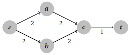
In this case, the only vital arc has weight 1, which is not the maximum weight edge.

(d) This is also false, and disproved by the same example above since the edge (c ,t) is part of the short-est path, but so are the weight 2 edges.

(e) To find a most vital arc, we first begin by locating the vital nodes of the graph. The vital nodes are the nodes that are contained in every shortest path from s to t . Note that a vital arc must necessarily come out of a vital node, otherwise there would be an alternate shortest path that avoided it. We’ll start by running Dijkstra’s algorithm from s. We will also run Dijkstra’s algorithm from t with all edges in the graph reversed. This gives us all shortest paths beginning at s and all shortest paths ending at t . Then we consider the subgraph G' that consists only of edges that are part of any shortest path. An edge (u, v) is on some s − t shortest path if and only if

δ(s,u) + w(u, v ) + δ(v,t ) = δ(s,t ),

which we can check using the results of the two invocations of Dijkstra.

This new graphG' must be acyclic since shortest paths will not contain cycles. To determine whether a vertex is part of every shortest path, we will compute for each vertex u ∈ V , the number of paths from u to t in G . This can be done with the following dynamic programming algorithm in O(V +E) time.

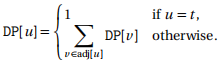
We will see more algorithms like this for directed acyclic graphs in the Week 10 lecture. Finally, we know that a vertex u is contained in all shortest paths if and only if DP[u] = DP[s], i.e. the number of shortest paths from u is equal to the total number of shortest paths, which means it must be in all of them.

Next, for each vital node we just discovered, we check the distance to t via every one of its out-going edges. This can be achieved by using the results of the Dijkstra’s algorithms we ran earlier. Specifically, if we are at vertex u, then the distance to t via the edge (u, v) is

δ(s,u) + w(u, v) + δ(v,t).

If the node has only one outgoing edge, then that edge is a vital arc whose removal disconnects s and t , hence it increases the distance by ∞. Otherwise, we take the two shortest distances d1 and d2 out of these. If they are equal, then there is no vital arc from this node, since either of these edges could replace the other as they achieve equally short paths. Otherwise, we have a vital arc that increases the distance by d2 − d1 . After checking all vital nodes, the largest distance increase that we discovered (if any) is a most vital arc.

We run two invocations of Dijkstra’s algorithm taking at most O((V + E)log(E)), the dynamic pro-gramming algorithm takes O(V + E), and checking every edge coming out of vital node takes O(E) time, so in total, this takes O((V + E)log(E)) time.

Problem 16. (Advanced) An improvement to the Bellman-Ford algorithm is the so-called “Shortest Paths Faster Algorithm”, or SPFA. SPFA works like Bellman-Ford, relaxing edges until no more improvements are made, but instead of relaxing every edge |V| − 1 times, we maintain a queue of vertices that have been relaxed. At each iteration, we take an item from the queue, relax each of its outgoing edges, and add any vertices whose distances changed to the queue if they are not in it already. The queue initially contains the source vertex s.

(a) Reason why SPFA is correct if the graph contains no negative-weight cycles.

(b) The algorithm described above will cycle forever in the presence of a negative-weight cycle. Add a simple condition to the algorithm to fix this and detect the presence of negative cycle if encountered.

(c) What is the worst-case time complexity of SPFA?

Solution

The proof of correctness for SPFA is pretty much exactly the same as for Bellman-Ford, so we will not write the whole thing formally. At the first iteration, all shortest paths consisting of at most 1 edge will be found by relaxing the edges out of s. Subsequently, all shortest paths of length at most two will be found when those vertices relax their outgoing edges, and so on. By induction, we can show that all shortest paths of length k will be relaxed after the shortest paths of length k − 1. SPFA essentially does the same thing as Bellman-Ford, but it avoids relaxing edges that will not make a difference.

In the presence of a negative weight cycle, SPFA will continue to add the vertices of the cycle to the queue forever. To stop this, we enforce that each vertex can only be removed from the queue at most n − 1 times. If a vertex is removed n times, this implies that the shortest path to it contains n +1 vertices since the queue always serves vertices in order of the number of edges on their shortest path, and in between multiple occurrences of the same vertex, the path length must increase.

Since we may remove each vertex from the queue n times, and each time we process every one of its edges, the amount of work done is at most O(V E ), the same as Bellman-Ford. Although this sounds bad, on average SPFA performs much better.

Problem 17. (Advanced) In this problem, we will derive a fast algorithm for the all-pairs shortest path problem on sparse graphs with negative weights1. We will assume for simplicity that the graph has no negative cycles, but the techniques here can easily be adapted to handle them. The key ingredient of the algorithm is based on the idea of potentials.

(a) Let d [v] : v ∈ V be the distances to each vertex v ∈ V from an arbitrary source vertex. Prove that for each edge (u, v) ∈ E

d [u] − d [v] + w(u, v) ≥ 0.

We define the quantity p[u] = d [u] as the potential of the vertex u.

(b) Give a simple algorithm to compute a set of valid potentials. Potentials should not be infinity for any vertex. Suppose now that we modify the weight of every edge (u, v) in the graph to

w'(u, v ) = p[u] − p[v] + w(u, v)

(c) Prove that a shortest path in the modified graph was also a shortest path in the original, unmodified graph.

(d) Deduce that we can solve the all-pairs shortest path problem on sparse graphs with negative weights in O(V² log(V)) time.

Solution

(a) This is a direct result of the triangle inequality. The triangle inequality states that

d [u] + w(u, v) ≥ d [v],

which must be true since if this quantity were less than d [v], then the path s  u → v would be shorter than the shortest path to v , a contradiction. Subtracting d [v] from both sides of the triangle inequality yields the desired result.

(b) A solution that almost works is to pick an arbitrary source vertex and run Bellman-Ford to compute the shortest distances. This will fail though if the source we pick can not reach every vertex since then some of the distances will be infinity. To correct this, we instead add a new vertex to the graph and connect it to every vertex with an edge weight of zero. We then run Bellman-Ford from this new vertex. By design, it is connected to every other vertex so none of the distances will be infinity. The resulting distances can be used as potentials.

(c) Consider a path in the modified graph v1 → v2 → ... → vk . Its total length will be

p[v1] − p[v2] + w(v1, v2) + p[v2] − p[v3] + w(v2, v3 ) + ... + p[vk−1] − p[vk] + w(vk−1, vk).

Observe that except for the first and last, the potentials all cancel since they appear as a positive term and then as a negative term immediately after. This leaves us with

p[v1 ] + w(v1, v2) + w(v2, v3) + ...+w(vk−1, vk) − p[vk].

Note that the only potentials left in the equation are of the first and last vertex, in other words, they do not depend on the path taken at all. The remaining terms simply constitute the path length of the path v1 → v2 → ... → vk in the original, unmodified graph, hence any shortest path in the modified graph is also a shortest path in the unmodified graph.

(d) With all of these ingredients, we can derive Johnson’s algorithm. First, we run Bellman-Ford from a new source vertex that connects to every other vertex in o