AREC 454/ECON 484 The Economics of Climate Change

AREC 454/ECON 484

The Economics of Climate Change

Prof. Alberini

Spring 2021

* Work individually, but it is okay to look up your class notes and google conversion factors for measurements, etc.

This project uses data collected from the US government to examine residential energy consumption. Specifically, we will be using data from the 2015 Residential Energy Consumption Survey (conducted by the US Energy Information Administration, an agency of the Department of Energy), plus other data collected by the US Environmental Protection Agency, to…

• Compute the CO2 emissions from electricity and heating and cooking fuels in US homes

• Identify heavy and low emitters

• Examine fuel poverty (which occurs when a household spends more than 10% of its income on electricity and fuels)

• Examine the incidence of a carbon tax, if one were imposed, on the various income groups

• Determine whether we would be better off with an economy-wide improvement in the energy efficiency of homes.

The data to be used for this project is in spreadsheet “RECS 2015 for AREC 454 project.xslx.”

This project can done in Excel, but you are more than welcome to use STATA, Matlab, R, or write your own Python code if you prefer.

Instructions are provided for Excel. Please be sure to install the “Data Analysis” package for Excel, as explained as the beginning of Homework 5.

Please read this document carefully before you get started.

1. DATA. The 2015 RECS collected extensive information about the dwelling, the household, and its use of electricity and other fuels. The survey resulted in a little over 6000 completed interviews, but in this assignment we are using only the records from those households that use electricity or gas (or both) for space heating. This results in N=4540 observations.

You will find these data in the sheet “Data” in the “RECS 2015 etc.” spreadsheet. A description of the variables is provided in the sheet “codebook.”

The most important variables for our purposes are

• kWh (total electricity usage in 2015 in kWh),

• cufeetng (total natural gas usage in 2015, in hundred cubic feet)

• electrprice (price of electricity in $/kWh)

• gasprice (price of natural gas in $/cubic foot)

• moneypy (income category from 1 to 8)

• hhincome (approx.. household income in 2015, in $, based on moneypy)

• hdd65 (heating degree days at the respondent’s location in 2015, using 65 °F as the base)

• cdd65 (cooling degree days at the respondent’s location in 2015, using 65 °F as the base)

• emissions (CO2 emissions in tons/MWh in the Census Division where the respondent lives)

2. CALCULATING EMISSIONS

Let us begin with calculating the CO2 emissions from consuming electricity. For each household, multiply kWh by emissions, and then divide by 1000 (there are 1000 kWh in one MWh). This produces the metric tons emitted in one year from the electricity consumed. Place this variable in col. BC.

Now calculate the emissions from burning natural gas (for space heating, heating water, and cooking), keeping in mind that one cubic meter of natural gas has 1.68 kg of CO2 and one cubic meter is 35.3147 cubic feet. Place this variable in col. BD and make sure that it is expressed in metric tons.

Then, create a new variable (to be placed in col. BE) which has the total CO2 emissions, namely the sum of those from electricity and those from natural gas.

Compute the share of total emissions from electricity, and place it in col. BF.

Q1. On average, which is the more important source of emissions from a home, electricity or natural gas? Is there evidence of variation across households?

Q2. Compute the average emissions of CO2 from electricity and from gas in each of the eight income groups. (Hint: in any empty cell, type AVERAGEIF(Q2:Q4541,1,BC2:BC54541) to compute the average electricity use for people in income group 1. Replace the “1” in the middle of that formula with 2, 3, etc. to do the other income groups. Repeat replacing BC with BD to examine the emissions from natural gas.)

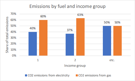
Create a bar chart that displays the average emissions from electricity and gas for each of these groups, and comment on the evidence. Do wealthier households create more or less emissions? Why?

(Hint. Your bar chart should look approximately like the one below, which is based on fictious data. Make sure the axes are labeled, there is a title for your chart, etc. Your chart needs to look professional.)

3. CALCULATING EXPENDITURES

Now calculate the total electricity bill (kWh*electrprice) and gasbill (cufeetng*100*gasprice), and place them in cols. BG and BH, respectively.

Q3. Compute the average electricity bill and average gas bill in each of the eight income groups. (Hint: see question Q2.) Again, create a bar chart that displays the average bills in each group, and comment on the evidence. Do the poorest income groups pay more or less for electricity and gas than the wealthiest income groups?

Now compute total energy expenditures (electricity bills + gas bills) as share of income (hhincome). Place this variable in col. BI.

Q4. Compute the shares of income in each of the eight income groups. (Hint: see question Q2.) Again, create a bar chart that displays the average share of income in each group spent on energy, and comment on the evidence.

A household is regarded as energy poor when its bills are more than 10% than income. Create an “energy poor” dummy using this definition and place this variable in col. BJ.

Q5. What is the percentage of “energy poor” households in this sample?

4. PRICE ELASTICITIES OF DEMAND

We are now getting ready to estimate an electricity demand function and a gas demand function. Copy kWH, cufeetng, electrprice, gasprice, totsqft_en, hdd65, cdd65, aircond, elwarm, elwater, elfood, ugwarm, ugwater and ugcook to a new sheet, and label this sheet “regressions.”

Create a new variable (lkwh) equal to the natural log of kWh, one (lgas) equal to the natural log of (cufeetng*100), one (lelectrprice) equal to the natural log of electricity price and one (lgasprice) that is the natural log of gasprice.

Create a new variable, lsqft, that is equal to the natural log of totsqft_en.

Then create a new variable, degreedays, that is equal to the sum of hdd65 and cdd65. Then create ldegreedays=ln(degreedays).

Q6. How are heating degree days calculated, and what are they supposed to measure? How are cooling degree days, and what are they supposed to measure? (Hint: google them, and trust the US Department of Energy’s or EIA’s explanation.)

Now we estimate a demand function for electricity. The fit of the regression is best when we work with the log of electricity consumption, log of price, etc.

Using the regression option in the “data analysis” tab (go to the data tab), run a regression where the dependent variable is lkWh and the independent variables are lelectprice, lsqft, ldegreedays, aircond, elwarm, elwater, and elfood. Then answer questions Q7-Q9 about this regression.

Q7. The coefficient on lelectprice is interpreted as the price elasticity of electricity demand. What is the value you have obtained? Is this elasticity larger, smaller, or in line with what we have learned in this course?

Aircond, elwarm, elwater, and elfood are dummy variables, and are coded 0 when the household doesn’t have A/C, doesn’t use electricity for heating, doesn’t use electricity to heat water, and doesn’t use electricity for cooking, and 1 otherwise. Their coefficients are interpreted as follows: If, for example, the coefficient on elwarm was 0.35, it would mean that people that use electricity for space heating use [exp(0.35)-1]*100% more electricity that people that do not use electricity for space heating, i.e., almost 42% more.

Q8. Use this information to interpret the impact of using A/C, using electricity for space heating, using electricity for heating water, and using electricity for cooking on electricity consumption.

Q9. Based on the price elasticity of electricity demand, how much (percentage-wise) would the demand for electricity change if there was a 10% improvement in the energy efficiency of the electrical equipment in this sample’s homes? (Hint: rebound effect from our energy efficiency lectures.)

Now run a regress of lgas (dependent variable) on the independent variables lgasprice, lsqft, lhdd, ugwarm, ugwater, ugcook, where lhdd is the natural log of hdd65. (You will have to create this variable.)

Q10. Are the signs of the coefficients on the independent variables from the gas regressions the ones you were expecting?

5. CARBON TAX AND SCC

Table 1 displays the Social Cost of Carbon values calculate by the federal government. Select the values for a 2.5% discount rate, and convert them to 2015 $.

Table 1. Social Cost of Carbon, 2007 US$

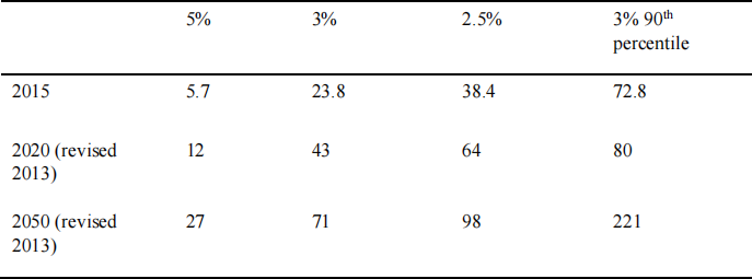
Q11. Compute what the carbon tax per kWh of electricity would have been in 2015 for each household in the sample, if it had been set equal to the SCC as calculated for 2015 (and expressed in 2015 dollars).

Compute the mean, min and max carbon tax per kWh.

Compute the mean carbon tax per kWh faced by the households in each Census Division.

Q12. Compute the total carbon tax that would have been paid by the household (=carbon tax per kWh, times kWh consumed), and the share of income that it represents. Then display the average total tax paid and the average share of income for each income group in a bar chart. Comment on the evidence.

6. THE ART AND COMMUNICATION OF CLIMATE CHANGE

Prepare a simple, on-page flyer to explain to a household why the world must cut emissions, what they should expect if a carbon tax is introduced, and how the household can reduce its tax payments (perhaps by reducing electricity and gas consumption, making homes more energy efficient, etc.). Be as creative as you wish. It is okay to find graphics and ideas online.