Computational Finance MATLAB Project

Computational Finance

MATLAB Project

Assume the stock price S(t) paying a continuous dividend yield q follows the following geometric Brownian motion:

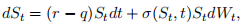
where r is the risk free interest rate and W is a Wiener process under the risk-neutral probability measure. Assume that the local volatility function σ(St, t) has been calibrated with the form

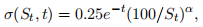
We know that the price of an option, V (S, t), on the above stock satisfies the Black-Scholes PDE:

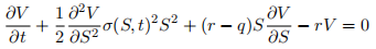
In this project you will price a standard European PUT option using both Finite Difference and Monte Carlo Methods subject to certain boundary conditions.

The aim of this project is to use the following pricing parameters, spot price S0 = £100, risk-free rate r = 3%, dividend yield q = 5%, time to maturity T = 1.0 year, and = 0.30 in the local volatility function. Using these parameters, solve the Black-Scholes PDE numerically to price a European PUT option at the two strike prices K = £80 and K = £120 by means of

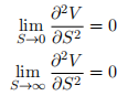
(1) Explicit finite differences
(2) Implicit finite differences
(3) Crank-Nicolson finite differences

Since there is no analytic solution to the PDE, you need to compare the results from the finite difference methods with the prices calculated from Monte Carlo simulation.

        You will need to turn in the following five items:

1. A maximum two page report (file format PDF) discussing the following (NOTE: there should be NO CODE in the written report!):

(a) (20% of project mark) Discuss proper domain and boundary conditions you should use in the finite difference schemes based on the properties of the option and the boundary conditions.

(b) (10% of project mark) For each of three finite di↵erence schemes, compare the prices with several different grid sizes with those from the Monte Carlo methods and report the convergence properties of each scheme.

(c) (10% of project mark) In the case of the explicit finite difference scheme demonstrate numerically by testing different grid sizes that the scheme is conditionally stable and find the condition for ∆t and ∆S under which the scheme would be stable.

2. The following four MATLAB scripts (NOTE: code which does not execute will be given zero credit):

(a) (15% of project mark) A single explicit.m script which executes the explicit finite differences method. More then one file should not be used. All functions should be self-contained in the explicit.m file.

(b) (15% of project mark) A single implicit.m script which executes the implicit finite differences method. More then one file should not be used. All functions should be self-contained in the implicit.m file.

(c) (15% of project mark) A single crank.m script which executes the Crank-Nicolson finite differences method. More then one file should not be used. All functions should be self-contained in the crank.m file.

(d) (15% of project mark) A single monte_carlo.m script which executes the Monte Carlo scheme with antithetic sampling. More then one file should not be used. All functions should be self-contained in the monte_carlo.m file.

        Each of the marks in the coding tasks will be split as follows: 60% for accuracy of the computation, and 40% for coding style, clarity of the code, and comments within the code.

        This project will contribute 40% towards the final mark for the module. Submit your work by uploading it in Moodle by 23:55 on Sunday, 12 April 2020. Submit the code as a single compressed .zip file containing exactly 5 files, the 4 Matlab (.m) files and the maximum two page report (as PDF). All five files should reside in a single parent directory, whose name should contain your name and student code.

        Unless approved exceptional circumstances apply (if you need to claim the exceptional circumstances, please refer to the exceptional circumstances procedure), late submissions will incur a penalty according to the formula:

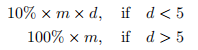
where m is the maximum mark that can be awarded for this assignment, and where d is the number of days or part days that the assignment is late, i.e. according to the standard university rules for late submission of assessed work. It is advisable to allow enough time (at least one hour) to upload your files to avoid possible congestion in Moodle before the deadline. In the unlikely event of technical problems in Moodle please email your .zip files to [email protected] before the deadline.

        It may prove impossible to examine projects that cannot be unzipped and opened, and run on computer lab machines directly from the directories created by unzipping the submitted .zip files. In such cases a mark of 0 will be recorded. It is therefore essential that all project files and the directory structure are tested thoroughly on computer lab machines before being submitted in Moodle. It is advisable to run all such tests starting from the .zip files about to be submitted, and using a different lab computer to that on which the files have been created.

NOTE: Submitted files that are archived/compressed with the RAR compression tool will receive an automatic 0.