STATS 415 Final Project
STATS 415 Final Project
Due by 11:59pm on April 18, 2021
1 Overview
In this project, you will apply what we have learned in STATS 415 to build predictive models based on a realifinancial dataset. The main goal is to predict the forward return of a target asset (Asset_1) based on the historical price series of the target asset and other two assets (Asset_2 and Asset_3). You will be given minutely prices of the three assets over a year, which correspond to T = 524, 160 rows in the csv file we provided.
The project has two parts: a basic part and an advanced part:
• In the basic part, there are six problems, each worth 10 points and having standard solutions. Two problems require you to submit your outputs to Canvas, which are then assessed by our Online Judge (OJ). The other problems require you to present your analysis and results in your project report, which are graded manually.
• The advanced part is worth 40 points. There you are given full freedom to build your predictive models. You need to submit a prediction function to Canvas; then our OJ will assess and report its performance on a testing dataset that is withheld from you. The ranking of a team depends on the out-of-sample correlation r of their model. You will receive 10 points as long as your team makes a valid submission and will receive full points once r ≥ 5%. We will consider giving extra bonus points to top teams depending on their performance. The specific details of the bonus points will be given after the final project is due.
Everyone within a team receives the same score for the final project and can submit results or code to the OJ for the entire team. Each OJ-graded problem allows three submissions per day per team, and only the highest score will be counted toward the grade. Therefore, please start early and exploit every opportunity to hit a higher score! During the final project, you will be updated with your team’s current ranking based on your state-of-theart result every 24 hours.
2 Basic part
2.1 Backward returns
For any t, h ∈ N+, define the h-min backward return at time t as:
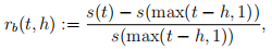
where s(t) denotes the price at time t. Load final project.csv in R. Calculate the 3-min, 10-min and 30-min backward returns of all the three assets at t = 1, . . . , T. Create a dataframe with columns named in the form of Asset_i_BRet
2.2 Rolling correlation
Given two times series  , the w-min backward rolling correlation between
  and
and  at time t0 is defifined as

where  is the sample correlation. Calculate the (21 ∗ 24 ∗ 60)-minute (3 weeks) backward rolling correlation of 3-min backward returns of each pair of the three assets at t = 1, 2, . . . , T. Create a dataframe with column names in the form of Rho_i_j, which corresponds to the rolling correlation between Asset i and Asset j, and where i < j. The resulting dataframe should have 524,160 rows and 3 columns. Export the dataframe to a csv file named as corr.csv, and submit it ot our OJ to verify its correctness. Please round all the entries of the dataframe to four decimal places; the maximum file size to upload is 15MB. (Hint: The rolling correlation can be computed in an incremental manner, given that the rolling window is shifted by only one minute at each step.)
2.3 Linear regression
The h-min forward return at time t is defined as:
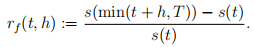
Fit a linear regression to predict rf (t, 10) of Asset 1 using rb(t, 3), rb(t, 10), rb(t, 30) of the three assets you calculated in Section 2.1 as features. Hence, you have 9 features in total in your linear model. Use the first 70% data as training data and the last 30% data as testing data. Are the backward returns of Assets 2 and 3 significant in predicting the forward return of Asset 1? Report the in-sample and out-of-sample correlation between your prediction ˆrf (t, 10) and true response rf (t, 10). Also plot the three-week backward rolling correlation between ˆ rf (t, 10) and rf (t, 10). Is this correlation structure stationary over the year?
2.4 KNN
Run KNN by using the same features and response variable as in Section 2.3 with K = 5, 25, 125, 625, 1000. Use the first 70% data as training data and the last 30% data as validation data. Plot the training and validation MSE against K. Find the best K based on the validation MSE and generate prediction for the whole year. Report the in sample and out-of-sample correlation between your prediction and true response.
Note that here we use the validation approach instead of cross validation (CV) to tune K, because we should not use future data for training and past data for validation.
2.5 Ridge and LASSO
Consider backward returns in more time horizons. Calculate

for all the three assets. Use these returns as features to fit Ridge and LASSO regression to predict rf (t, 10) of Asset 1. Use the first 70% data as training data and the last 30% data as validation data. Use the validation MSE to seek the best tuning parameter in LASSO and Ridge, and generate the corresponding prediction for the whole year. Report the in-sample and outof-sample correlation between your prediction and true response.
2.6 Principle component regression (PCR)
Run PCR with the same features and response as in Section 2.5. Use the fifirst 70% data as training data and the last 30% data as validation data. Use the validation MSE to seek the optimal number of principal components to include in PCR and generate the corresponding prediction for the whole year. Report the in-sample and out-of-sample correlation between your prediction and true response.
3 Advanced part
You have tried some basic features and models in the previous problems. Now you are in position to derive new features based on the dataset and develop your own sophisticated statistical models.
Your task is to write a R function prediction() that takes a dataframe of past one-day minutely price data of Assets 1, 2 and 3 (i.e., a 1440-by-3 numeric dataframe) as input, and that returns the prediction of the 10-minute forward return of Asset 1 at the last minute of the input dataframe as output. Conceptually speaking, this prediction function is your estimate of the regression function fˆ. Note that there SHOULD NOT be any model fitting inside this function. Rather, you should train your model based on the given data OUTSIDE this function, and extract the fitted model to build prediction().
You should submit two files to our OJ: prediction.R and model.RData. The R script prediction.R includes the function prediction. Feel free to include other utility functions in prediction.R. The file model.RData includes all the objects you need to build your prediction function, e.g., the optimal choice of tuning parameters, the estimate of the coefficients in the linear model, etc. The size limit for both files is 32MB. The OJ will apply your prediction function to the testing dataset that covers half a year and return to you the correlation between your prediction and true forward return. Your prediction function will be called for around 10 thousand times, and the total time limit for this is 10 minutes. Therefore, please ensure that your prediction function is both accurate and fast!
In terms of package usage, feel free to use all the packages in the lab materials. Please do not use any packge that has not appeared in the lab materials.
3.1 Some tips regarding code submissions
1. Prior to submitting your code, see if you can call your prediction function 10,000 times within five minutes on your local computer. If not, then please simplify your model or code.
2. You don’t have to load model.RData or the packages you need inside the prediction function. Instead, do them outside the prediction function. This can avoid repeatedly loading the model objects and save substantial amount of time.
3. It is recommended that you put rm(list=ls()) in the beginning of your script prediction.R to refresh the local environment of the OJ.
2021-04-19