CMDA 3634 SP2021                            Parallelizing the Wave Equation with MPI                            Project 04

Project 04: Parallelizing the Wave Equation with MPI

Version: Current as of: 2021-04-12 13:54:50

Due:

– Preparation: 2021-04-20 23:59:00

– Coding & Analysis: 2021-05-05 23:59:00 (24 hour grace period applies to this due date.)

Points: 100

Deliverables:

– Preparation work as a PDF, typeset with LaTeX, through Canvas.

– All code through code.vt.edu, including all LaTeX source.

– Project report and analysis as a PDF, typeset with LaTeX, through Canvas.

Collaboration:

– This assignment is to be completed by yourself or by your group.

– For conceptual aspects of this assignment, you may seek assistance from your classmates. In your submission you must indicate from whom you received assistance. 

– You may not assist or seek assistance from others that are not in your group on matters of programming, code design, or derivations.

– If you are unsure, ask course staff.

Honor Code: By submitting this assignment, you acknowledge that you have adhered to the Virginia Tech Honor Code and attest to the following:

I have neither given nor received unauthorized assistance on this assignment. The work I am presenting is ultimately my own.

References

● MPI:

– Eijkhout book on MPI and OpenMP: http://pages.tacc.utexas.edu/~eijkhout/pcse/html/index.html

– MPI Quick Reference: http://www.netlib.org/utk/people/JackDongarra/WEB-PAGES/SPRING-2006/mpi-quick-ref.pdf

Code Environment

● All necessary code must be put in your class Git repository.

– If you are working with a partner or group, you will need to create a new git repository to work from.

– You must add, at minimum, the instructor and the GTAs as developers to this repository. If you need assistance from a ULA you may need to add them as well.

● Use the standard directory structure from previous projects.

● All experiments will be run on TinkerCliffs.

● Be an ARC good citizen. Use the resources you request. Use your scratch space for large data.

● Any scripts which are necessary to recreate your data must be in the data directory.

DO NOT INCLUDE VIDEO FILES OR LARGE NUMBERS OF IMAGE FILES OR IN YOUR GIT REPOSITORY!

● Your tex source for project preparation and final report go in the report directory.

● Remember: commit early, commit often, commit after minor changes, commit after major changes. Push your code to code.vt.edu frequently.

● You must separate headers, source, and applications.

● You must include a makefile.

● You must include a README explaining how to build and run your programs.

Requirements

For this project, you have the opportunity to work in teams of two or three. Your teammates must be in your section. If you choose to work with a team:

● You may collaborate on the Preparation assignment, but you must submit your own writeup, in your own words!

● You will complete and submit Coding & Analysis assignment jointly, with one minor exception detailed below.

Preparation (20%)

1. Write a work plan for completing this project. You should review the coding and analysis sections, as well as the remaining course schedule. Your work plan should include a description of the steps you think will be necessary to complete the required tasks, as well an estimate of the time that each task will take. Be sure to account for resource requirements. To properly answer this question, you will need to take some time and think through the remainder of the assignment.

If you have choose to work with a team, identify them here and sign up for a group on Canvas. In this case, your work plan must include additional details describing how you are going to work together, what collaboration tools you will use, a division of labor, how frequently you plan to meet (remotely), whose code you will start from, etc.

For continued safety, you are not permitted to meet in person!

All meetings must use Zoom, FaceTime, Hangouts, Slack, etc.

2. In Labs 06 and 07, we used 1D domain decomposition to distribute the N data in the vectors. Here is the formula we used to find the number of entries (Nr) to be assigned to each rank r of P processors:

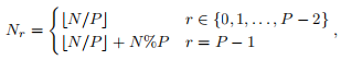
where % is the mod operator and bN/Pc means N/P rounded down to the nearest integer. However, this decomposition is prone to load imbalance.

(a) How bad is the load imbalance if N = 1001 and P = 1000? What about if N = 1999 and P = 1000?

(b) In the case for, N = 1999 and P = 1000, what is the optimal distribution of work?

(c) Develop a better formula for distributing such data. You will use this formula to help distribute the rows of your computational grids. In your new formula, the difference between the largest amount of work assigned to one rank and the smallest assigned to one rank may not be greater than 1. Also, the relationship Nr ≥ Nr+1 must hold for all r (except r = P − 1, obviously).

3. Disregarding the header (which has negligible size), for a solution that is ny × nx = 100, 001 × 100, 001, how large will a single solution file be on disk? Give your answer exactly, in bytes, and approximately, in the largest reasonable unit (KB, MB, GB, etc.).

4. For each of the following configurations, estimate how many CPU hours will be charged. These computations will be relevant in tasks 2-4 of the analysis.

(a) A batch script requesting 4 entire nodes (512 total CPUs) for the following:

> mpirun -np 1 ./wave_timing 10001 3 4 1.0 250

Run time: 460s

(b) A batch script requesting 4 entire nodes (512 total CPUs) for the following:

> mpirun -np 512 ./wave_timing 10001 3 4 1.0 250

Run time: 1.25s

(c) A batch script requesting 8 entire nodes (1024 total CPUs) for the following:

> mpirun -np 1024 ./wave_timing 10001 3 4 1.0 100

Run time: 0.3s

(d) A batch script requesting 8 entire nodes (1024 total CPUs) for the following:

> mpirun -np 1024 ./wave_timing 100001 3 4 1.0 100

Run time: 26s

5. What information needs to be stored in the 2D array data structure to operate in a domain decomposed environment? You may assume that the domain will be decomposed using a 1D domain decomposition in the y dimension, only. Also, assume that we will be writing output files in parallel. Address, at minimum, the following:

● For the wave simulation, how large should the halo/padding region be? 

● Which dimension(s) should be padded?

● What information is necessary to map the internal data to the global grid coordinate system.

● What other information do you think will be useful?

Coding (60%)

For this project you may start from your solution to project 2 or project 3, or my solution to project 2. If you are working with a team you may start from either of your solutions, or merge them.

● The source code for your solution is to be submitted via GitLab.

● This project is to be written in the C language, using MPI.

● You must include a Makefile in your code directory. This makefile should include targets for each executable you are required to produce, a target to compile all executables, and a clean target to remove intermediate build files and executables.

● You must include a readme file, explaining how compile and run your code.

● You are provided some source code in array 2d io.h/c, found in the materials repository. This includes an example parallel file writer as well as one that you will need to complete.

Tasks:

1. Modify your makefile to enable compilation with MPI.

2. Modify your timing, image generation, error calculation, and animation programs to use MPI. Be sure to update the timing to use MPI tools – there should be no remnants of OpenMP.

3. Modify your 2D array data structures for operation in a domain decomposed environment. Be sure to include all necessary information to map the internal data to the global grid coordinate system. We will decompose the problem using a 1D domain decomposition in the y dimension.

● Be sure to update your memory management routines (allocation, deallocation, etc.). Your allocation function should perform the actual domain decomposition, so it will need access to the MPI communicator.

● Data must be optimally distributed, using the approach developed in Task 2 of the Preparation phase.

● Complete the routine compute subarray size in array 2d io.h/c, implementing the formula you developed in Task 2 of the Preparation phase. This is required for one of the provided routines and will be helpful elsewhere.

4. Implement a routine to perform a halo exchange for a domain-decomposed computational grid. For full credit, you must use the non-blocking send/receive operations.

5. Complete the provided stub (write float array dist mpiio in array 2d io.h/c) to use MPI I/O to write your wavefields to a single file, in parallel. An implementation that does not use MPI I/O is provided for testing purposes and so that you may complete other aspects of the project.

6. Use MPI to parallelize your function for computing the error norm.

7. Update your functions for evaluating the standing wave and computing one iteration of the simulation to work with distributed grids. Be sure to ensure that the halo regions are properly updated. There will be a minimum of two rows per subdomain.

8. Write SLURM submission scripts for generating the results in the analysis section. Use the solutions to Task 4 of the preparation to inform the construction of your scripts.

9. If you are working in a group of 3, complete one of the three additional tasks listed at the end of the project.

Analysis (20%)

● Your report for this project will be submitted via Canvas. Tex source, images, and final PDFs should be included in your Git repositories.

● All timings and analysis should be from experiments on TinkerCliffs.

● I suggest that you run each of the experiments as separate jobs on TinkerCliffs. Use the early experiments to estimate how long the later ones might take.

● Unless otherwise specified, use α = 1, mx = 17, and my = 27.

● You should assume that n = nx = ny for the global problem.

Tasks:

1. Use outputs from your image and error calculation programs to generate images and plots to demonstrate that your parallel code is working correctly for P = 64 MPI tasks. Pick a large enough problem to be interesting, but small enough that you can save images or build any animations you want to share.

2. Run a strong scalability study for n = 10001, nt = 250, and P = 1, 2, 4, 8, 16, 32, 64, 128, 256, and 512 for your wave equation simulation.

(a) You should run a small number of trials per experiment.

(b) Create plots of both the run-times and speedup. Remember, these are a function of P.

(c) Does this problem good strong scalability? Justify your claim and explain why you think you observe this behavior.

3. Run a weak scalability study for n = 2501 (for P = 1), nt = 250, and P = 1, 2, 4, 8, 16, 32, 64, 128, 256, and 512 for your wave equation simulation.

(a) You should run a small number of trials per experiment.

(b) Create plots of both the run-times and speedup. Remember, these are a function of P.

(c) Does this problem good weak scalability? Justify your claim and explain why you think you observe this behavior.

4. For P = 1024 (all of the cores on 8 nodes of TinkerCliffs), time the execution of nt = 100 iterations of your wave equation simulator for n = 2,501; 5,001; 10,001; 25,001; 50,001; 75,001; and 100,001.

● Plot your results as a function of N = nx × ny. On separate lines on the plot, include your results from similar questions for Projects 1, 2, and 3. You may either re-run the experiments from Project 1 and 2 for 100 iterations or rescale the results so that they are equivalent to 100 iterations.

● Look at your timing results from Projects 1, 2, and 3. Use MATH to estimate how many CPU hours it would take to run 100 simulation iterations with n = 100, 001 based on each project’s timings (three different predictions). For Project 3, use your P = 64 data.

● How many CPU hours did the n = 100, 001 case take for this project?

● What conclusions can you draw from this semester long experiment?

● How might you use this knowledge when working on future projects?

5. If you are working in a group of 3, complete the additional analysis tasks corresponding to the additional task you chose for the Coding section.

6. Evaluate your working style on this project.

● If you worked on this project with a team, in the identified separate Canvas assignment, give 4 bullet points discussing your collaboration in detail.

– State each team members specific contributions.

– What challenges and successes did you experience with collaboration tools?

– How did the workload break down between you and your team and were you able to follow the work plan?

– How satisfied were you with both your effort and work ethic and your team’s effort and work ethic?

This question will be graded individually, and we reserve the right to assign different grades on the overall assignment in the event of an imbalance in collaborative effort.

● If you did not work on this project with a team, in this submission, give 3 bullet points discussing your work process in detail.

– How well were you able to follow your work plan?

– How satisfied were you with your effort and work ethic?

– How do you think things would have gone differently if you had chosen to worked with a team?

Extra Credit Task: The Wave Equation with a Point Source

● Additional Coding Tasks

1. Implement a new function for simulating a wave solution with a point source. The results of this simulation will look like a ripple on a pond. This simulation works exactly the same way as the the ones we’ve performed using the standing waves, except for the following:

– The equation is

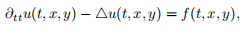
where f is the source function.

– The time-update in the simulation has one additional term,

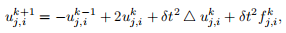
where  is the source field.

– The point source is located at the point (xs, ys). For this project, we will place the source at the grid point closest to that point. We will represent that grid point by the indices (js, is).

– The source function is,

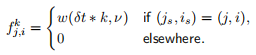
C source code for evaluting w(t, ν) is provided in the materials repository.

– Instead of initializing with the standing wave, the initial conditions are

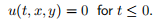
Your implementation should work with your domain decomposed structures.

● Additional Analysis Tasks

1. Using at least 8 MPI tasks and a domain sized at least n = 501, create an animation showing propagation of your point source. You should run the simulation long enough that the wave reflects off of the domain boundaries a couple of times.

Start with (xs, ys) = (0.5, 0.5) and ν = 10 Hz, but experiment with the source location to find an interesting location and frequency.

Upload you animation to Canvas or google drive.

Additional Tasks for 3-member Teams

Option A: MPI + OpenMP

● Additional Coding Tasks

1. Modify your code to use both MPI and OpenMP simultaneously.

● Additional Analysis Tasks

1. Re-run the experiment from Task 4 of the Analysis, once using P = 512 MPI tasks with 2 OpenMP threads per task and once using P = 256 MPI tasks with 4 OpenMP threads per task. (This preserves the total of 1024 total processors.) Plot your results with Task 4. Do you see an improvement on the pure MPI case? You should experiment futher to see if more OpenMP threads yields improved performance.

To run these experiments, use the following mpirun command as an example:

> mpirun -np 256 --map-by ppr:32:node --bind-to L3cache -x OMP NUM THREADS=4

./your timing program arg1 arg2 ...

Option B: 3D Simulations

● Additional Coding Tasks

1. Modify your code so that you can do 3D simulations. You should create a separate copy of your code and programs for this. It will be more challenging to have 2D and 3D contained inside one code. You should still do a 1D domain decomposition, but in the z dimension this time.

The initial condition (through the standing wave function) extends naturally:

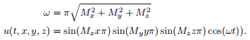
The Laplacian also extends naturally (k is the z index and s is the time index), assuming δx = δy = δz:

The stable time-step in 3D is (for α ≤ 1):

● Additional Analysis Tasks

1. Create some 3D visualizations to demonstrate that your program is working correctly in a distributed memory environment. You may consider plotting some 2D slices or 3D renderings. Use enough processors to perform a small scalability study.

● Hints

– These problems get large quickly (100003 = 100 ∗ 1000002 , so keep n under 1001.

Option C: 2D Domain Decompositions

● Additional Coding Tasks

1. Modify your code to use 2D domain decompositions instead of 1D domain decompositions. The modified code should support arbitrary and different numbers of processors in the x and y dimensions. You will need to modify your halo exchange to use separate communication buffers for each side and dimension.

● Additional Analysis Tasks

1. Compare the run times for the n = 10001 and P = 256 using the following numbers of processors in the x and y dimensions. The fifirst configuration is equivalent to a 1D decomposition in the y dimension, the last is equivalent to a 1D decomposition in the x dimension.

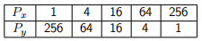
Which configuration performs best? Use your knowledge of the system and the problem to explain why you think this is the case?

● Hints

– Look into MPI’s Cartesian communicators for creating the 2D structure. For example, MPI Cart create, MPI Cart coords, and MPI Cart shift may be useful.

Development and Debugging Hints

● Test the analysis tasks on small examples to be sure that they work prior to submitting the big test jobs.

● Start by implementing the domain decomposition and testing it on your distributed form of the standing wave evaluation. You have a functional array writer that you can use to test. You should get the same output for P = 1, 2, 3, . . . .

● Use the provided array writer to compare output to your MPI I/O based writer. These outputs should be identical.

● Your original array writer can be used to write out individual subdomains. This can be useful for debugging.

● If you print debug output, print each worker’s rank first. You can sort by the rank to see each worker’s execution path.

● You can use the animation program to create small examples that can help you visualize if your domain decomposition and halo exchange are working correctly. Look for artifacts around the subdomain boundaries.

● After evaluating or updating a solution, ensure that the halo regions are properly updated.

● Think about which subdomains have to handle the boundary conditions.