FIT1045/FIT1053 (S1-2021)

(Advanced) Algorithms and programming in Python

Programming Assignment

Assessment value: 22% (10% for Part 1 + 12% for Part 2)

Due: Week 6 (Part 1), Week 11 (Part 2)

Prepared by Dr. Buser Say and Dr. Mario Boley

Objectives

The objectives of this assignment are:

• To demonstrate the ability to implement algorithms using basic data structures and operations on them.

• To gain experience in designing an algorithm for a given problem description and implementing that algorithm in Python.

• To explain the computational problems and the challenges they pose as well as your chosen strategies and programming techniques to address them.

Submission Procedure

You are going to create a single Python module file ann.py based on the provided template. Submit a first version of this file by the due date of Part 1, Friday 11:55pm of Week 6. Submit a second version of this file by the due date of Part 2, Friday 11:55pm of Week 11.

Important Note:   Please ensure that you have read and understood the university’s policies on plagiarism and collusion available at http://www.monash.edu.au/students/policies/academic-integrity.html. You will be required to agree to these policies when you submit your assignment. A common mistake students make is to use Google to find solutions to the questions. Once you have seen a solution it is often difficult to come up with your own version. The best way to avoid making this mistake is to avoid using Google. You have been given all the tools you need in workshops. If you find you are stuck, feel free to ask for assistance on the Ed discussion forums, ensuring that you do not post your code.

Marks and Module Documentation

This assignment will be marked both by the correctness of your module and your analysis of it, which has to be provided as part of your function documentation. Each of the assessed functions of your module must contain a docstring that contains, in this order:

1. a one line short summary of what the function is computing,

2. a formal input/output specification of the function,

3. some usage examples of the function (in doctest style),

4. a paragraph explaining the specific problems that need to be solved by this function, and your overall approach in tackling these problems, and

5. a paragraph explaining the specific choices of programming techniques that you have used.

        For example, if scaled(row, alpha) from Lecture 6 was an assessed function its documentation in the submitted module could look as follows:

def scaled(row, alpha):

""" Provides a scaled version of a list with numeric elements.

Input : list with numeric entries (row), scaling factor (alpha)

Output: new list (res) of same length with res[i]==row[i]*alpha

For example:

>>> scaled([1, 4, -1], 2.5)

[2.5, 10.0, -2.5]

>>> scaled([], -23)

[]

This is a list processing problem where an arithmetic operation has to be carried out for each element of an input list of unknown size. This means that a loop is required to iterate over all elements and compute their scaled version. Importantly, according the specification, the function has to provide a new list instead of mutating the input list. Thus, the scaled elements have to be accumulated in a new list.

In my implementation, I chose to iterate over the input list with a for-loop and to accumulate the computed scaled entries with an augmented assignment statement (+=) in order to avoid the re-creation of each intermediate list. This solution allows a concise and problem-related code with no need to explicitly handle list indices. 

"""

res = []

for x in row:

res += [alpha*x]

return res

        Beyond the assessed functions, you are highly encouraged to add additional functions to the module that you use as part of your implementation of the assessed functions. In fact, such a decomposition is essential for a readable implementation of the assessed function, which in turn forms the basis of a coherent and readable analysis in the documentation. All these additional functions also must contain a minimal docstring with the items 1-3 from the list above. Additionally, you can also use their docstrings to provide additional information, which you can refer to from the analysis paragraphs of the assessed functions. Finally if you are taking FIT1053, you must include your answer to the last question in each part as a comment in your submission file.

        This assignment has a total of 22 marks (10 + 12) for FIT1045 students and 25 marks (11 + 14) for FIT1053 students, and contributes to 22% of your final mark.1 For each day an assignment is late, the maximum achievable mark is reduced by 10% of the total. For example, if Part 1 of the assignment is late by 3 days (including weekends), the highest achievable mark on that part of the assignment is 70% of 10, which is 7. Assignments submitted 7 days after the due date will normally not be accepted.

        Mark breakdowns for each of the assessed functions can be found in parentheses after each task section below. Marks are subtracted for inappropriate or incomplete discussion of the function in their docstring. Again, readable code with appropriate decomposition and variable names is the basis of a suitable analysis in the documentation.

Overview

Inspired from the human brain, artificial neural networks (ANNs) are a type of computer vision model to classify images into certain categories.2 In particular, in this assignment we will consider ANNs for the task of recognising handwritten digits (0 to 9) from black-and-white images with a resolution of 28x28 pixels. In Part 1 of this assignment you will create functions that compute an ANN output for a given input, and in Part 2 you will write functions to “attack” an ANN. That is, to try to generate inputs that will fool the network to make a wrong classification.

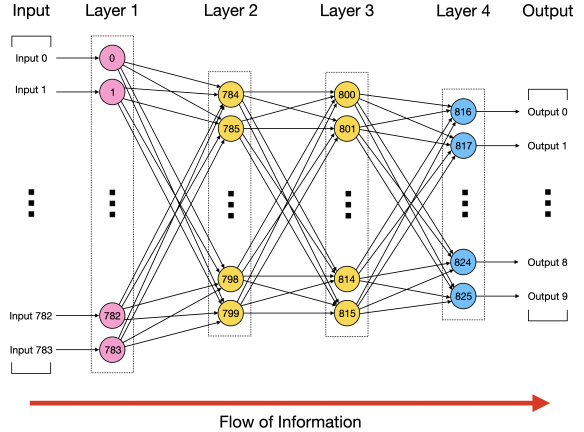
Figure 1: Visualization of the Artificial Neural Network (ANN) that will be used in this assignment. The ANN visualized has four layers in total with 784 vertices in its first layer (i.e., one for each pixel, coloured in with pink), 10 vertices in its last layer (i.e., one for each digit, coloured in with blue), and 16 vertices in its remaining layers (i.e., coloured in with yellow). The red arrow visualizes the layer-by-layer information flow through the ANN.

        Figure 1 illustrates the general build-up of an ANN for this task. The network receives the 784 pixels of the input image in the form of a list of pixel values where the two possible values are 0 for white and 1 for black. Then it performs a computation by passing the data through several layers of neurons and finally producing a list of outputs with 10 elements. These 10 elements contain a numerical score for each possible digit (0 to 9) that correspond to how likely the network thinks that the input image shows the specific digit.

        For instance, the image in Figure 2 would be fed to the network as the list:

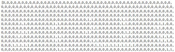
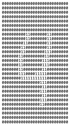
Figure 2: Visualization of the image with a resolution of 28x28 pixels that is classified to be number 4 by the ANN.

The output list could then be

[-2.166686, -5.867823, -1.673018, -4.412667, 5.710625, -6.022383, -2.174282, 0.378930, -2.267785, 3.912823]

corresponding to the fact that the network thinks that the most likely digit shown is a 4 but 9 also not being unlikely.

        Aside from solving the digit classification task which serves as an intuitive demonstrative example, ANNs are mainly designed to solve critical tasks such as making cancer diagnosis from mammogram images, driving vehicles from sensory input etc. Therefore, it is extremely important to ensure the safety of such ANNs. One common practice of ensuring the safety of an ANN is to attack it, which is typically carried out by minimally modifying the input (e.g., the image) to see if the ANN makes a different prediction (e.g., digit classification).3

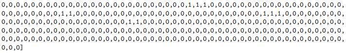
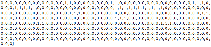
        For instance, Figure 3 visualizes an adversarial image generated by attacking the ANN visualized in Figure 1 based on the original input image that is previously visualized in Figure 2. That is, when the adversarial image is fed to the network as the list:

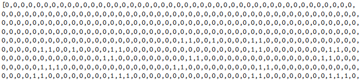
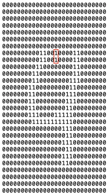
Figure 3: Visualization of the adversarial image with a resolution of 28x28 pixels that is classified to be number 9 by the ANN. Note that the only difference between the adversarial image and the original image visualized in Figure 2 is the two pixels that are highlighted by the red square.

the ANN could be led into thinking the adversarial image is more likely to be number 9 (instead of number 4) based on its following output list

[-2.102353, -5.111125, -1.799243, -4.036013, 4.205424, -5.937777, -2.942028, 0.794603, -2.199816, 4.538266].

Part 1: ANN Inference (10 marks in total + 1 mark for FIT1053)

As indicated in the overview figure (i.e., Figure 1), an ANN is organised in layers, and each layer consists of a number of “neurons” that we refer to as vertices. When classifying an input image, the input data flows first to the vertices in the input layer (i.e., coloured in with pink in Figure 1), from there on through a number of inner layers (i.e., coloured in with yellow in Figure 1), and finally through an output layer (i.e., coloured in with blue in Figure 1) that computes the final scores. The vertices in the input and the output layers work a bit differently than the inner layers. So let us focus on those first. The vertices in the input layer are extremely simple: they just forward the value of a single input pixel to all vertices of the subsequent layer.

Single Output Vertex (1 mark)

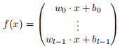
The output vertices are a little more complicated: given an input vector x = (x0, . . . , xd−1) of some dimension d, they compute a linear function:

defined by a d-dimensional weight vector of w and a single number b called the bias. Note that we use the usual notation w · x to denote the dot product of w and x, i.e., the sum w0x0 + · · · + wd−1xd−1.

        Write function linear(x, w, b) that can be used to compute the output of an individual vertex in the output layer by adhering to the following specification:

Input: A list of inputs (x), a list of weights (w) and a bias (b).

Output: A single number corresponding to the value of f(x) in Equation 1.

For instance, for input vector x = (1.0, 3.5), weight vector w = (3.8, 1.5) and bias b = −1.7 the output of a single vertex (i.e., the output of vertex 4 in Figure 4) is computed as:

>>> x = [1.0, 3.5]

>>> w = [3.8, 1.5]

>>> b = -1.7

>>> linear(x, w, b)

7.35

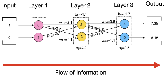
Figure 4: Visualization of the example ANN that has three layers in total with 2 vertices in its first layer (i.e., coloured in with pink), 2 vertices in its last layer (i.e., coloured in with blue), and 2 vertices in inner layer (i.e., coloured in with yellow). The red arrow visualizes the layer-by-layer information flow through the ANN.

Output Layer (1 mark)

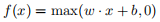
Now to compute the combined output of the whole output layer that consists of l vertices, we just have to compute the joint output of many linear functions. That is, given the weight vectors w0, . . . wl−1, biases b0, . . . , bl−1 of the individual vertices and the input data x flowing in from the preceeding layer, the output of the output layer is described by the function:

Write function linear layer(x, w, b) that can be used to compute the output of the whole output layer by adhering to the following specification:

Input: A list of inputs (x), a table of weights (w) and a list of biases (b).

Output: A list of numbers corresponding to the values of f(x) in Equation 2.

For instance, for input_vector x = (1.0, 3.5), weight matrix 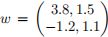 and biases b = (−1.7, 2.5) the combined output of the whole output layer (i.e., the output of vertices 4 and 5 in the example ANN that is visualized in Figure 4) is computed as:

>>> x = [1.0, 3.5]

>>> w = [[3.8, 1.5], [-1.2, 1.1]]

>>> b = [-1.7, 2.5]

>>> linear_layer(x, w, b)

[7.35, 5.15]

Inner Layers (1 mark)

Next we need to compute the output of the vertices in the inner layers. Individually, the output of a single vertex that is located in an inner layer is computed by the following piecewise linear function:

for a given input vector x, weight vector w and bias b. Therefore, given the weight vectors w0, . . . wl−1, biases b0, . . . , bl−1 of the individual vertices and the input data x flowing in from the preceeding layer, the output of an inner layer is described by the function:

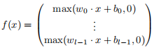
Write function inner_layer(x, w, b) that can be used to compute the output of an inner layer by adhering to the following specification:

Input: A list of inputs (x), a table of weights (w) and a list of biases (b).

Output: A list of numbers corresponding to the values of f(x) in Equation 4.

For instance, for input vector x = (1, 0), weight matrix  and biases b = (−1.1, 4.2) the combined output of the whole inner layer (i.e., the output of vertices 2 and 3 in the example ANN that is visualized in Figure 4) is computed as:

>>> x = [1, 0]

>>> w = [[2.1, -3.1], [-0.7, 4.1]]

>>> b = [-1.1, 4.2]

>>> inner_layer(x, w, b)

[1.0, 3.5]

Full Inference (2 marks)

Finally, we can put everything together to compute the output of the whole ANN (e.g., scores) given some input vector (e.g., pixels). Specifically, the output of the ANN is computed layer-by-layer starting from the input layer, continuing with the inner layer(s) and ending with the output layer. That is, the output of the vertices in the input layer must be computed first, which is then used in the output computation of the vertices in the inner layer(s), which is finally used in the output computation of the vertices in the output layer.

        Write function inference(x, w, b) that can be used to compute the output of an ANN by adhering to the following specification:

Input: A list of inputs (x), a list of tables of weights (w) and a table of biases (b).

Output: A list of numbers corresponding to output of the ANN.

The function inference behaves as follows for the example ANN (i.e., visualized in Figure 4) with weight matrices , bias matrix  and input vector x = (1, 0):

>>> x = [1, 0]

>>> w = [[[2.1, -3.1], [-0.7, 4.1]], [[3.8, 1.5], [-1.2, 1.1]]]

>>> b = [[-1.1, 4.2], [-1.7, 2.5]]

>>> inference(x,w,b)

[7.35, 5.15]

        Next, we will focus on implementing functions that read in and store data from text files.

Reading Weights (1 mark)

The weights of the ANN will be stored in a text file and must be read in and stored. For example, the weights of the example ANN that are visualized in Figure 4 (also included in ‘example_weights.txt’) will have the following format:

#

2.1,-3.1

-0.7,4.1

#

3.8,1.5

-1.2,1.1

where the character # is used to separate two adjacent weight matrices.

        Write function read weights(file_name) that can be used to read in the weights of the ANN by adhering to the following specification:

Input: A string (file_name), that corresponds to the name of the file that contains the weights of the ANN.

Output: A list of tables of numbers corresponding to the weights of the ANN.

For example, the function read_weights behaves as follows:

>>> w_example = read_weights(‘example_weights.txt’)

>>> w_example

[[[2.1, -3.1], [-0.7, 4.1]], [[3.8, 1.5], [-1.2, 1.1]]]

>>> w = read_weights(‘weights.txt’)

>>> len(w)

3

>>> len(w[2])

10

>>> len(w[2][0])

16

Reading Biases (1 mark)

Similarly, the biases of the ANN will be stored in a text file and must be read in and stored. For example, the biases of the example ANN that are visualized in Figure 4 (also included in ‘example_biases.txt’) will have the following format:

#

-1.1,4.2

#

-1.7,2.5

where the character # is used to separate two adjacent bias vectors.

        Write function read biases(file_name) that can be used to read in the biases of the ANN by adhering to the following specification:

Input: A string (file_name), that corresponds to the name of the file that contains the biases of the ANN.

Output: A table of numbers corresponding to the biases of the ANN.

For example, the function read biases behaves as follows:

>>> b_example = read_biases(‘example_biases.txt’)

>>> b_example

[[-1.1, 4.2], [-1.7, 2.5]]

>>> b = read_biases(‘biases.txt’)

>>> len(b)

3

>>> len(b[0])

16

Reading the Image File (1 mark)

The image in Figure 2 visualizes a black-and-white image of a handwritten digit using zeros for white pixels and ones for black pixels over 28x28 pixels (i.e., 784 in total). Write function read_image(file_name) that can be used to read in the image visualized by Figure 2 by adhering to the following specification:

Input: A string (file name), that corresponds to the name of the file that contains the image.

Output: A list of numbers corresponding to input of the ANN.

For example, the function read image behaves as follows:

>>> x = read_image(‘image.txt’)

>>> len(x)

784

        Finally, we will solve the handwritten digit classification task.

Output Selection (1 mark)

The computed scores by the ANN will be used to predict what number is represented in the image. Specifically, given a vector of computed scores x = (x0, . . . , xd−1) of some dimension d, the predicted number i will be the index of score xi with the highest score. Write function argmax(x) that can be used to return the index of an element with the maximum value.

Input: A list of numbers (i.e., x) that can represent the scores computed by the ANN.

Output: A number representing the index of an element with the maximum value in the list x. If there are multiple elements with the same maximum value, the function should return the minimum index (e.g., see the example below).

For example, argmax behaves as follows for input list x:

>>> x = [1.3, -1.52, 3.9, 0.1, 3.9]

>>> argmax(x)

2

Number Prediction (1 mark)

Finally, write function predict number(image_file_name,weights_file_name,biases_file_name) that solves the handwritten digit classification task.

Input: A string (i.e., image_file_name) that corresponds to the image file name, a string (i.e., weights_file_name) that corresponds to the weights file name and a string (i.e., biases_file_name) that corresponds to the biases file name.

Output: The number predicted in the image by the ANN.

For example, predict number behaves as follows for file names ‘image.txt’, ‘weights.txt’ and ‘biases.txt’:

>>> i = predict_number(‘image.txt’,‘weights.txt’,‘biases.txt’)

>>> print(‘The image is number ’ + str(i))

The image is number 4

Additional Question for FIT1053 (1 mark)

Write a comment (i.e., using #) in the beginning of your ann.py file the answer to the following question. What does the ANN predict to be the third most likely number represented in the image that is visualized in Figure 2? Please explain how you came up with this conclusion.

Part 2: Adversarial Image (12 marks in total + 2 marks for FIT1053)

In this part of the assignment, you will write an algorithm that generates an adversarial image (e.g., Figure 3) to an ANN (e.g., Figure 1) based on an input image (e.g., Figure 2). More formally, you will solve the computational problem of minimally modifying the pixels of an input image such that the number classified by the ANN for the adversarial image is different than that of the input image.

    Let us start by defining what modifications are allowed to carry out an attack. For simplicity, you will only be allowed to modify pixels from 0 to 1 and from 1 to 0, and we will refer to this operation as flip.

Flip a Pixel (0.5 mark)

Write function flip_pixel(x) that can be used to flip a single pixel by adhering to the following specification:

Input: An integer (x) representing a pixel in the image.

Output: An integer representing the flipped pixel.

The function flip_pixel(x) must behave as follows:

>>> x = 1

>>> flip_pixel(x)

0

>>> x = 0

>>> flip_pixel(x)

1

        Next, the image that is represented as a list should be modified by flipping a single pixel.

Modify a List (0.5 mark)

Write function modified_list(i,x) that can be used to flip the pixel that is located at position i in list x by adhering to the following specification:

Input: A list of integers (x) representing the image and an integer (i) representing the position (i.e., index) of the pixel.

Output: A list of integers (x) representing the modified image.

For example, the function modified_list(i,x) behaves as follows for input list x and index i:

>>> x = [1, 0, 1, 1, 0, 0, 0]

>>> i = 2

>>> modified_list(i,x)

[1, 0, 0, 1, 0, 0, 0]

        Now that the basic operations to carry out an attack are covered, the next step is to measure the quality of an adversarial image.

Quality Computation (1 mark)

The quality of an adversarial image is measured by the total absolute pixel-by-pixel difference between the input image and the generated adversarial image. For example, for the input image that is visualized in Figure 2 and the adversarial image generated that is visualized in Figure 3, the quality would be 2.

        Write function compute_difference(x1,x2) that can be used to compute the total absolute difference between the adversarial image and the original image by adhering to the following specification:

Input: A list of integers (x1) representing the input image and a list of integers (x2) representing the adversarial image.

Output: An integer representing the total absolute difference between the elements of x1 and x2.

For example, the function compute_difference(x1,x2) behaves as follows for lists x1 and x2:

>>> x1 = [1, 0, 1, 1, 0, 0, 0]

>>> x2 = [1, 1, 1, 0, 0, 0, 1]

>>> compute_difference(x1,x2)

3

        Using the functions you have written previously (including the ones for Part 1), you can now start designing and implementing an algorithm that attacks the ANN given an input image. For example, let us first demonstrate below how to obtain and compute the quality of the adversarial image (i.e., Figure 3) to the ANN (i.e., Figure 1) given the input image (i.e., Figure 2)

>>> x1 = read_image(‘image.txt’)

>>> x2 = read_image(‘image.txt’)

>>> x2 = modified_list(238,x2)

>>> x2 = modified_list(210,x2)

>>> quality = compute_difference(x1,x2)

>>> print(‘The quality of the adversarial attack is ’ + str(quality))

The quality of the adversarial attack is 2

where x1 and x2 represent the input and the adversarial images as lists.

        Note that we still have not discussed how to select which indices to flip (e.g., 238 and 210 in the example above), so let us do that next.

Select a Pixel (5 marks)

The pixel that is to be flipped should be selected based on its overall impact on the output list of the ANN. For example, modifying pixel at position 238 produces the following output list

[-2.087871, -5.475471, -1.621999, -4.213924, 4.903939, -6.095823, -2.653019, 0.697776, -2.230024, 4.242473]

which decreases the score for number 4 by around 0.8.4 , while increasing the score for number 9 (i.e., the second most likely number) by around 0.3.5 Therefore the overall impact of flipping pixel at position 238 would be around 1.1.6

        Write function select pixel(x, w, b) that can be used to either (i) select which pixel to flip or (ii) conclude that no further modifications can be made (i.e., when the overall impact of flipping is negative for all pixels), by adhering to the following specification:

Input: A list of inputs (x), a list of tables of weights (w) and a table of biases (b).

Output: An integer (i) either representing the pixel that is selected to be flipped, or with value -1 representing no further modifications can be made.

For example, the function select pixel(x, w, b) can behave as follows for input list x, list of tables of weights w and table of biases b:

>>> x = read_image(‘image.txt’)

>>> w = read_weights(‘weights.txt’)

>>> b = read_biases(‘biases.txt’)

>>> pixel = select_pixel(x, w, b)

>>> pixel

238

>>> x = modified_list(pixel,x)

>>> pixel = select_pixel(x, w, b)

>>> pixel

210

Note that the behaviour of your algorithm will change depending on how function select pixel(x, w, b) is designed and implemented. You must clearly explain your design and implementation choices for function select pixel(x, w, b) in docstring.

        Before you write an algorithm that generates an adversarial image, you will first write a function that writes the list representation of the adversarial image into a file as a 28x28 image.

Write Image (1 mark)

Write function write image(x, file_name) that can be used to write the list x into a file with name file name as a 28x28 image by adhering to the following specification:

Input: A list of integers (x) representing the image and a string (file_name) representing the file name.

Output: Write out each pixel represented in the list x to a file with the name file_name as a 28x28 image.

For example, the function write_image(x, file_name) behaves as follows for input list x and file name file_name:

>>> x = read_image(‘image.txt’)

>>> x = modified_list(238,x)

>>> x = modified_list(210,x)

>>> write_image(x,‘new_image.txt’)

where the last line will produce a text file that is visualized in Figure 3.

        Finally, you will write a function that solves the adversarial image problem.

Adversarial Image (4 marks)

Write function adversarial image(image_file_name,weights_file_name,biases_file_name) that solves the adversarial image generation task.

Input: A string (i.e., image_file_name) that corresponds to the image file name, a string (i.e., weights_file_name) that corresponds to the weights file name and a string (i.e., biases_file_name) that corresponds to the biases file name.

Output: A list of integers representing the adversarial image or the list [-1] if the algorithm is unsuccesful in finding an adversarial image.

For example, adversarial_image can behave as follows for file names ‘image.txt’, ‘weights.txt’ and ‘biases.txt’:

>>> x1 = read_image(‘image.txt’)

>>> x2 = adversarial_image(‘image.txt’,‘weights.txt’,‘biases.txt’)

>>> if x2[0] == -1:

... print(‘Algorithm failed.’)

... else:

... write_image(x2,‘new_image’)

... q = compute_difference(x1,x2)

... print(‘An adversarial image is found! Total of ’ + str(q) + ‘ pixels were flipped.’)

...

An adversarial image is found! Total of 2 pixels were flipped.

Note that the behaviour of your algorithm will change depending on how function adversarial image(image_file name,weights_file_name,biases_file_name) is designed and implemented.    You must clearly explain your design and implementation choices for function adversarial_image(image_file_name,weights_file_name,biases_file_name) in docstring.

Additional Question for FIT1053 (2 marks)

Write a comment (i.e., using #) in the beginning of your ann.py file the answer to the following question. What is the worst-case complexity of solving the adversarial image problem optimally in terms of the input (i.e., image) size using the Big-O notation? Please explain how you came up with this result.