MTH 600: Project

Winter 2021

Instructor: Wei Xu                                            Office: VIC 709                                       e-mail: [email protected]

Office Hours:                                                    by appointment on Zoom

Due 11:59 pm April. 24 (Saturday), on D2L

IMPORTANT INFORMATION:

The delivery of this project includes following documents:

1. A detailed report that contains all relevant parts of the solutions (explanations, graphs, etc.).

2. Five Matlab .m files.

(a) Eur_Call_LVF_MC.m (function for the option pricing by the Monte Carlo method)

(b) Eur_Call_LVF_FD.m (function for the option pricing by the Finite Difference method)

(c) PriceTest.m (script to compute the option price with parameters given in Question 4 by Monte Carlo and Finite Difference method).

(d) myfun.m (function to compute the objective function and Jacobian matrix of F(x) in question 5.)

(e) Calibration.m (script to calibrate x1, x2, x3 of the LVF given the option prices in Question 5b).

All Matlab files have to be well documented. Most of the marks for programming questions are allocated for explanations of algorithms and discussions of results. If all you hand in is the listing of the “Raw Code” or “Raw Output” by itself, you will get poor marks. All coding should be done in Matlab/Octave (nicely commented). Moreover, please make sure that both PriceTest.m and Calibration.m can be run immediately in Matlab/Octave after typing the name into the prompt.

All files should be submitted online via D2L. Penalty for late submission is 10 marks per day (i.e., you will receive maximum 90 if you submit your assignment on April 25).

Project Question. (100 points)

A typical practice in finance is to estimate an option pricing model from market prices of options that are traded frequently (in other words, liquid options). The calibrated model can be used to hedge liquid options or price and hedge other (illiquid) exotic options on the same underlying. In this project, we will consider the calibration of a local volatility function (LVF) model in practice.

The LVF model assumes the stock price as

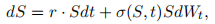
where . The European call option value is then the solution of the PDE

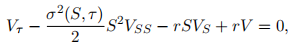
where is the time to maturity.

1. (10 points) Write the initial condition and boundary conditions for the above PDE.

2. (20 points) Write a pseudo-code for pricing the European call option at t = 0 by the Monte Carlo method. Implement the pseudo-code by Matlab with the following function interface. 

function V = Eur Call LVF MC(S0, K, T, r, x, M, N)

%

% Price the European call option of the LVF model by the Monte Carlo method

%

% Input

%   S0 – initial stock price

%   K – strike price

%   T – maturity

%   r – risk free interest rate

%   x – vector parameters for the LVF σ, [x1, x2, x3]

%   M – number of simulated paths

%   N – number of time steps, i.e., δt = T /N.

% 

% Output

%   V – European call option price at t = 0 and S0.

3. (20 points) Derive the computational scheme for the explicit method and write a pseudocode for the explicit method to solve (1) with the initial and boundary conditions. Implement the pseudo-code by Matlab with the following function interface.

function V0 = Eur Call LVF PDE(S0, K, T, r, x, Smax, M, N)

%

% Price the European call option of the LVF model by the explicit finite difference method.

%

% Input

%   S0 – initial stock price

%   K – strike price

%   T – maturity

%   r – risk free interest rate

%   x – vector parameters for the LVF σ, [x1, x2, x3]

%   Smax – upper bound of the stock price

%   M – number of stock price difference, i.e., δS = Smax/M

%   N – number of time steps, i.e., δt = T /N.

% 

% Output

%   V 0 – European call option price at t = 0 and S0.

4. (20 points) Compute the results from the Monte Carlo method with S0 = 1, K = 1, T = 0.25, r = 0.03, x = [0.2, 0.001, 0.003], M = 10, 000 and N = 100. Compare the results from the explicit finite difference with S0 = 1, K = 1, T = 0.25, r = 0.03, x = [0.2, 0.001, 0.003], Smax = 3, M = 30 and N = 100.

5. (30 points) The main purpose of this question is to familiarize you with the calibration problem and its challenges.

Assume that the initial market prices V0 mkt(Kj , Tj ), j = 1, 2, · · · , m, are available; here (Kj , Tj ) denotes the strike and expiry of the j-th option.

Assume that V0(Kj , Tj ; x) denotes the initial value of an option with strike Kj and Tj under a LVF model described by a set of parameters x = (x1, x2, · · · , xn). In the quadratic local volatility model (1), the model parameters are (x1, x2, x3).

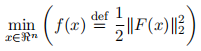
The model which best fits the market option prices can be estimated by solving the following nonlinear least squares problem

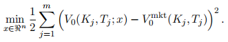
Let F(x) denote the vector of model option value errors from the market prices:

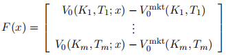
Vector F(x) : is a nonlinear function of the model parameter x ∈ and the calibration problem (2) is equivalently formulated as

A nonlinear least squares problem (3) can be solved by a special optimization method such as the Levenberg-Marquardt method, the Gauss-Newton method, or a general method for nonlinear unconstrained optimization problems.

Optimization methods for nonlinear least squares problems typically exploit the special structure of the gradient and Hessian of the function . They typically require computation of the Jacobian matrix of F(x)

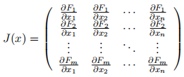
One difficulty in solving the nonlinear least squares calibration problem (2) is that it is not easy to compute the Jacobian matrix J(x) explicitly. Instead, a finite difference approximation of the Jacobian matrix can be computed.

(a) (10 points) Write a matlab function to return F(x), and J, if necessary, for any given x. Your Matlab function must return, in the second output argument, the Jacobian matrix J at x. Note that, by checking the value of nargout, you can avoid computing J when your Matlab function is called with only one output argument (in the case where the optimization algorithm only needs the value of F but not J). You can use either Monte Carlo method or Finite difference method implemented in previous questions to evaluate V0(K, T, x). The set of call option prices  given below:

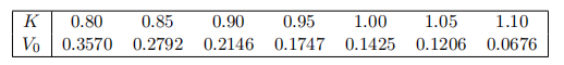
All of these options have expiry in three months. The other parameters for the option are the same as the ones in question 4.

function [F,J] = myfun(x)

F = ...                            % Objective function values at x

if nargout > 1                 % Two output arguments

    J = ...                         % Jacobian of the function evaluated at x

End

Compute J using finite difference approximation as described in class.

(b) (20 points) Use Matlab function lsqnonlin with LevenbergMarquardt as the choice of the optimization method to estimate the unknown coefficients x for the LVF model from the set of call option prices given above. You can set the options for optimization as follows

options = optimoptions(’lsqnonlin’,’SpecifyObjectiveGradient’,true);

options.Algorithm = ’levenberg-marquardt’;

options.Display = ’iter’;

Perform the computation with the following starting points respectively:

• x0 = [0.2; 0.0; 0.0];

• x0 = [0.2; 0.1; 0.01];

For each starting point, report the estimated parameter set x∗ and the calibration error . For each computed x* , plot the given implied volatilities and the implied volatilities of the corresponding option values from the computed x* . Comment on the extent to which the matlab program is successful in solving the calibration problem.