Continuous Assessment 1 of Foundations of Financial Computing

(23, Mar 2021–9, April 2021)

Instruction

1. This assignment is a formal component of Assessments as defined in the MTH116 Module Handbook, which will contribute 15% toward your final module grade (Please find the latest information about weights of the components of assessments in the updated module handbook on the LMO.)

2. This project assignment is required to be completed individually. Any academic misconduct including plagiarism, copying, collusion and dishonest use of data will be investigated according to Academy Integrity Policy (available on e-Bridge under the heading ”Policies and Regulations”). We strongly encourage you to submit before the deadline, otherwise, it may affect the fifinal marks of your report according to ”Code of Practice on Assessment”.

3. There are two major parts (Part I and Part II) in this assessment (in total 4 pages in this document). Please read carefully about the requirements. You are also provided with several files: template.m, b3.mat,C3.mat,and other helpful documents.

4. Submission deadline: 5pm Friday, 9 April 2021. Submission must be made via the Learning Mall.

What you will need to submit

1. Please use the file template.m provided for your work. For each problem in PART I, you’ll need to create a few lines of Matlab script that can solve the question. You just need to show your Matlab script, and need NOT to display results of the code. Please provide proper comments (as shown in the file template.m for question 1) to make the code easy to understand.

2. For problems in PART II, you need to create several functions that do the work for questions 2, 3, and 4 as displayed in the template. Comment your code in the functions appropriately to make it readable. You are again advised to use the file template.m as a template to write the functions. Make sure your M-file works in the end. In other words, when we test your M-file by putting the name of your file in the MATLAB command window, MATLAB will be able to do all the work for the questions automatically.

3. After you have completed all the tasks (PART I and PART II), please put all scripts into the template file. Re-name the file with your own name, e.g. JoeBiden.m. Include your name and ID number at the top in the file as well. You will then need to submit your file via the submission link on the LMO by 5pm 9 April 2021.

PART I (40 Marks in total).

The LF model is an important model in the economics. It considers the consumption and production balance of a whole country or region. In the model there are n industries producing n different products such that the input equals the output or, in other words, consumption equals production. One distinguishes two models:

● Open model: some production consumed internally by industries, rest consumed by external bodies.

   Problem: Find production level if external demand is given.

● closed model: entire production consumed by industries.

   Problem: Find relative price of each product.

The notation of consumption matrix A can be used to describe the relations that a sector has with all the other sectors. The matrix A will be a matrix such that each column vector represents a different industry and each corresponding row vector represents what that industry inputs as a commodity into the column industry.

For example, The consumption matrix A below represents the relationships between the industries of Farming, Construction, and Clothing.

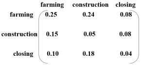
Figure 1: The consumption matrix

● The entry a11 holds the number of units the farmer uses of his own product in producing one more unit of farming. The entry a21 holds the number of units the farmer needs of construction to produce one more unit of farming. The entry a31 holds the number of units the farmer needs of clothing to produce one more unit of farming.

● The entry a12 holds the number of units that the builder needs from the farmer to produce one more unit of building .The entry a22 holds the number of units the builder needs of construction to produce one more unit of construction. The entry a32 holds the number of units the builder needs of clothing to produce one more unit of construction.

● The entry a13 holds the number of units of farming that the tailor needs to produce one more unit of clothing. The entry a23 holds the number of units of construction that the tailor needs to produce one more unit of clothing. The entry a33 holds the number of units of clothing that the tailor needs to produce one more unit of his own product.

Denote the external demand vector by b (The demand vector b is the amount of product the consumers will need). Represent the equilibrium production vector by x, i.e., the total production that will be needed to satisfy the external demand vector b. Then the L-F model is formulated:

b = x − Ax.

Note that in the case of closed model, we have b = 0.

Questions: Please write down proper Matlab scripts to solve the following 4 questions.

1. (5 Marks) For the consumption matrix displayed in Fig 1. If the external demand vector is . Find the equilibrium production vector x1.

2. (5 Marks) Suppose the external demand vector becomes , what is the new equilibrium production vector (denoted by x2) ? Find the difference between the new equilibrium with the old vector. How much extra product must each sector provide (denoted by d).

3. (5 Marks) Suppose the consumption matrix is changed into

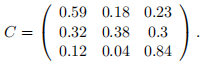
Can you find an equilibrium vector to solve the closed model? What can you tell more about the equilibrium vector?

4. (25 in total) We now consider a more complex economic model in 1947, where the economy is divided into 25 sectors:

1. Agriculture and Fisheries

2. Food and Kindred Products

3. Textiles and Apparel

4. Lumber, Wood, and Furniture

5. Paper, Printing, and Publishing

6. Chemicals, Petroleum Products, Rubber

7. Leather and Leather Products

8. Stone, Clay, and Glass Products

9. Primary Metals

10. Fabricated Metal Products

11. Machinery (non-electric)

12. Electrical Machinery

13. Motor Vehicles

14. Other Transportation Equipment

15. Miscellaneous Manufacturing

16. Coal, Gas, and Electric Power

17. Transportation Services

18. Trade

19. Communications

20. Finance, Insurance, Real Estate

21. Business Services

22. Personal and Repair Services

23. Miscellaneous Services

24. New Construction and Maintenance

25. Undistribute

4-1. (10 Marks) The consumption matrix is stored in matrix C3 in file C3.mat (the unit is million US dollar) and the external demanding vector is stored in b3 in file b3.mat. Find the equilibrium production vector for the consumption matrix C3 and demanding vector b3.

4-2. (15 Marks) If the final demand for motor vehicles increases by one billion dollars, how much will the production of fabricated metal products have to increase to compensate?

PART II (60 Marks in total)

Preliminary analysis of the stock prices of Tesla Inc. in 2020. The stock price of Tesla, Inc. increased dramatically in 2020. This has made its CEO Elon Musk be the riches man in the world according to Forbes. This question requires you to do some preliminary analysis of the stock prices of Tesla, Inc. in 2020. The data analysis is required to be done with MATLAB.

1. (5 Marks) Get the daily stock prices of Tesla, Inc. in the entire year of 2020 (From Jan 1st 2020 to Dec 31st 2020) from e.g. yahoo finance.

2. (10 Marks) Import the data into MATLAB using the command importdata ()

3. (30 Marks) Use MATLAB (i.e. write MATLAB commands to let your computer do for you) to find out the answers to the following questions:

(a) (15 Marks) On which day did the adjusted close price of Tesla reach its maximum 2020 ? What is the maximum value ? How many days does it take for the adjusted close price increase from its minimum to maximum ? What is the average increase per day during this period ?

(b) (15 Marks) Assume the increase of price in a day is defined as a difference, i.e.

adjusted close price − open price

on that day. On which day did the price of Tesla increase most rapidly? What are the maximum increases? Answer these two questions again if the increase of price is defined as a rate, i.e.

(adjusted close price − open price)/(open price)

4. (15 Marks) Using the adjusted close price of Tesla in each day. Use the plot command to make a 2-D line plot to show the trend of this price in each day of 2020. Customize your plot with regard to the following aspects:

● Title. Add a title to this plot.

● Axis Labels. Add appropriate labels to the axes of this plot.

● Axis Limits. If necessary set these limits appropriately.

● Axis Tick Values and Labels. Use dates as tick labels of the horizontal axis to make your plot more informative.

● Mark both the maximum and minimum prices on the plot.

As of this writing, the stock price of Tesla is 654.87$. To compare this price with all the prices in 2020, make a horizontal line of 654.87$ on the same plot. Use different line styles to distinguish the two lines if necessary.

Finally, export your graphic to a file for future reference.

You may need to do some self-study on the following topics:

● Add Title and Axis Labels to Chart

● Specify Axis Limits

● Specify Axis Tick Values and Labels

● Create Line Plot with Markers

using Matlab Help function.