Dynamical systems

1. Bifurcation and indices   Consider the dynamical system

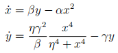
where , , and are real parameters.

a) Show that one can write the system (1) using a single dimensionless parameter a multiplying the term corresponding to in . What is the form of the parameter a?

b) Find all fixed points of the dimensionless version of the system (1). Determine the conditions on the parameter a for which the different fixed points exist. If you did not solve subtask a), then put = =  = 1 and = a.

c) For the four values , plot the dimensionless flow (1) and all existing fixed points. Label each fixed point with its index.

d) Based on the fixed points in subtask b) and their indices in subtask c), address the following tasks without evaluating the stability exponents

i. Find all bifurcations where fixed points are created or destroyed.

ii. Is the index conserved in the bifurcations?

iii. Discuss the possible types of fixed points that can be involved in the bifurcations.

2. Conservative systems   Consider the dynamical system

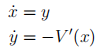
where V (x) is given by the figure below.

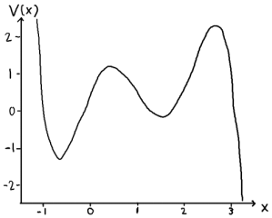
a) Sketch the phase portrait of this system and briefly explain how you obtain it. If you want to make the sketch by hand, you can either scan your solution, or take a photo of it.

b) For each fixed point you find in subtask a) do the following

i. highlight its stable and unstable manifolds in the phase portrait.

ii. indicate all regions in your sketch that contain closed orbits.

iii. verify that the indices of all closed orbits come out as expected.

The following subtasks are unrelated to subtasks a) and b)

c) Sketch the phase portrait of a dynamical system that has exactly one fixed point and two closed orbits.

d) Construct the equations for  and w in a dynamical system that has an integral of motion .

3. Lyapunov exponents of the damped driven pendulum   Consider the damped driven pendulum

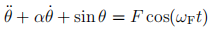
where α is a dimensionless damping rate, and where F and ωF are magni-tude and angular frequency of an external periodic forcing. Assume that all parameters are positive and that θ is periodic on .

a) Write Eq. (2) as a dynamical system of dimensionality 3 for the coor-dinates (, , ) where .

b) For the case F = 0, analytically determine the Lyapunov exponents of the system in subtask a) as functions of α. Explain the signs of the Lyapunov exponents.

c) Let F = 1 in what follows. For each of the values = {0.1, 0.5, 2}, numerically integrate the system in subtask a) from an arbitrary initial condition. Make one plot showing the long-time asymptotes of the three resulting trajectories in the (, ) plane for a range of large .

d) Based on asymptotic trajectories similar to those in subtask c), use the method of successive QR-decompositions to numerically evaluate the Lyapunov exponents of the system in subtask a) as functions of α in the range 0 ≤ ≤ 5 and address the following tasks

i. Make a plot containing your resulting Lyapunov exponents to-gether with the analytical result (for F = 0) from subtask b).

ii. Do your results agree?

iii. If there are ranges where the results agree, explain why F does not matter much in these ranges.

iv. If there are ranges where the results do not agree, explain what happens in these ranges.