CW1: An Unknown Signal

Originally by: Michael Wray & Davide Moltisanti

1 Introduction

The year is 1983, the strategy of Detente (de-escalation via verbal agreement) has failed. Both the United States of America and the Soviet Union have been stockpiling nuclear weapons and recent political events have brought the world on the cusp of total annihilation. As an operator for a nuclear early warning device you receive an unknown signal...

2 Task

In this coursework you will be given example points which follow an unknown signal. You will be required to reconstruct the signal and give the resulting error. Your mark will be based on a report you write about the code, submitted to the “Data-Driven Computer Science Coursework” submission point. You will also submit the code as a single python file to “Code submission point”. We will check that the code satisfies the basic requirements (in the implementation section) and for plagarism, but we won’t assess its performance.

You are required to work on this coursework individually. You may consult with your peers on the concepts and spirit of the assignment/solution, but you may not exchange code or passages of text for the report.

The deadline is April 30th at noon UK time.

3 Implementation

Your final solution will use the linear least squares regression code that you have created in the worksheets which will need to be extended in order to cope with non-linear curves. Your solution should:

• Read in a file containing a number of different line segments (each made up of 20 points)

• Determine the function type of line segment,

– linear

– polynomial with a fixed order that you must determine

– unknown nonlinear function that you must determine

• Use maximum-likelihood/least squares regression to fit the function

• Produce the total reconstruction error

• Produce a figure showing the reconstructed line from the points if an optional argument is given.

Note: All Code written for the least squares regression sections must be written by yourself. You can use anything in the Python standard library (https://docs.python.org/3/library/) but the only external libraries your so-lution should use are:

• Numpy

• Pandas

• Matplotlib

e.g. scipy, sk_learn and torch are not permitted.

4 Report

The aim of this report is to demonstrate your understanding of methods you used, the results you obtained and your understanding of issues such as over-fitting. The report should be no more than 4 pages long, using no less than 11 point font, with at least 2 cm margins. You should include:

• Equations for linear regression.

• Justification for your choice of polynomial order. Include plots.

• Justification for your choice of unknown function. Include plots.

• Description of your proceedure for selecting between linear/polynomial/unknown functions, accounting for overfitting.

5 Train/Test Files

The input files are Comma Separated Value (CSVs) which consists of two columns for the x and y dimensions respectively. Each input file will be split into different line segments each made up of 20 different points, so the first 20 points correspond to the first line segment, 21-40 the second line segment etc.

Two consecutive line segments may/may not follow the same trend. A line seg-ment will follow a linear, polynomial or another unknown function. An example train file is given below (basic_2.csv):

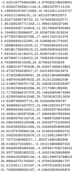
This corresponds to 40 points of x and y co-ordinates which make up the two different line segments of the file. Test files could consist of any number of line segments (i.e. longer than adv_3.csv) as well as have large amounts of noise.

6 Input/Output

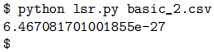
We expect a program called lsr.py (not a jupyter notebook) which will be run as follows:

After execution your program should print out the total reconstruction error, created by summing the error for every line segment, followed by a newline character:

Additionally, to further understand and validate your solution we wish for your program to be able to visualise the result given an optional parameter, --plot. This is only to visually check that your solution is working (and so that you can save plots for your report). For example, running:

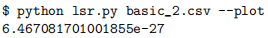
Will also show the following visualisation:

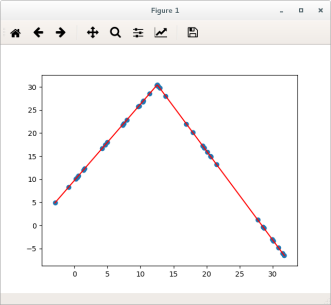
Note the presence of both the original points (blue dots) and fitted line segments (red lines).

7 Hints/Notes

• We have provided you a utilities file which contains two functions: load_points_from_file and view_data_points. The first will load the data points from a file and re-turn them as two numpy arrays. The second will visualise the data points with a different colour per segment. Feel free to copy-paste this code into your final solution (it will be excluded from plagarism checks).

• The error you need to calculate is the sum squared error.

• Regardless of the number of segments your program needs to only output the total reconstruction error.

• The test files will include points approximating line segments generated from the three functions mentioned above, i.e. linear, polynomial or the unknown function.

• The order of the polynomial (and the form of the unknown function) will not change between different files/segments.

• Having a very low error might not be the correct answer to a noisy solution, refer to overfitting in the lecture slides.

• You probably shouldn’t use regularisation (the coursework is designed under the assumption that you’ll use the simplest possible function classes to mitigate overfitting, rather than regularisation).