CSC242 Intro to AI Project 3: Uncertain Inference
CSC242 Intro to AI
Project 3: Uncertain Inference
In this project you will get some experience with uncertain inference by implementing some of the algorithms for it from the textbook and evaluating your results. We will focus on Bayesian networks, since they are popular, well-understood, and well-explained in the textbook. They are also the basis for many other formalisms used in AI for dealing with uncertain knowledge.
Requirements
1. You must design and implement a representation of Bayesian Networks for vari-ables with finite domains, as seen in class and in the textbook.
2. You must implement the Inference by Enumeration algorithm for exact inference described in AIMA Section 14.4.
3. You must implement the Rejection Sampling and Likelihood Weighting algorithms for approximate inference described in AIMA Section 14.5.
4. You must implement a method for reading networks from files, following a format known as XMLBIF.
Each of these are described in more detail in subsequent sections.
Background
Recall that a Bayesian network is a directed acyclic graph whose vertices are the random variables {X} U E U Y, where:
• X is the query variable
• E are the evidence (observed) variables
• Y are the unobserved (or hidden) variables
The inference problem for Bayesian Networks is to calculate P(X | e), where e are the observed values for the evidence variables. That is, inference in Bayesian networks involves computing the posterior distribution of the query variable given the evidence. In other words, inference in Bayesian networks involves computing a probability for each possible value of the query variable, given the evidence.
In general, from the definition of conditional probability and the process of marginaliza-tion, we have that:
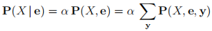
And for a Bayesian network you can factor that full joint distribution into a product of the conditional probabilities stored at the nodes of the network:
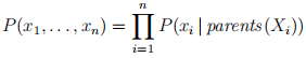
Therefore, for a Bayesian network:
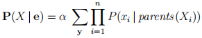
Or in words: “a query can be answered from a Bayesian Network by computing sums of products of conditional probabilities from the network” (AIMA, page 523). These equa-tions are the basis for the various inference algorithms for Bayesian networks.
Designing an Implementation of Bayesian Networks
You will need to implement a representation of Bayesian networks and several inference algorithms that use the representation. Before you can do that, you need to understand what these things are. Really understand.
So: what is a Bayesian network?
THINK ABOUT THIS YOURSELF NOW, THEN READ ON.
DID YOU THINK ABOUT IT?
REALLY?
WITH A WHITEBOARD OR A PIECE OF PAPER IN FRONT OF YOU?
IF SO, READ ON.
I thought first of a directed graph. A directed graph is a set of nodes (vertices) with directed edges between them. Everyone in CSC242 should be comfortable with graphs. If you’re a bit rusty on them, either look at your notes from CSC172 or go find the textbook used in CSC173 online (Chapter 9 is on graphs).
In a Bayesian network, each node in the graph is associated with a random variable. Each random variable has a name and a domain of possible values. We will assume finite domains for this project, although you are welcome to try problems involving con-tinuous domains also if you like.
Each node in the graph also stores a probability distribution. Root nodes (with no par-ents) store the prior probability distribution of their random variable. Non-root nodes store the conditional probability distribution of their random variable given the values of its parents: P(Xi | parents(Xi)).
Next question: What is a Bayesian network inference problem?
THINK ABOUT THIS YOURSELF NOW, THEN READ ON.
A Bayesian network inference problem involves computing the distribution P(X | e), where X is the query variable and e is an assignment of values to the evidence variables (note the similarity with our terminology from Unit 2).
The answer to a Bayesian network inference problem is a posterior distribution for the query variable given the evidence. That is, for each possible value of the query vari-able, it’s the probability that the query variable takes on that value, given the evidence. Another way of thinking about distributions is that they are a mapping from values of a variable to probabilities—the probability that the variable takes on that value, given the evidence. Note that distributions must satisfy the axioms of probability.
A Bayesian network inference problem solver takes a Bayesian network and an infer-ence problem (query and evidence, using variables from the network), and has one or more methods that compute and return the posterior probability distribution of the query variable given the evidence. The solver may have additional properties or parameters if needed.
Implementing Bayesian Networks
With the background fully understood, start by designing the main elements of your program. This should be done abstractly: define what the different pieces are and what they need to do but not how they do it. An important aspect of this is the relationships between the pieces.
If you will be programming in Java, I strongly recommend using Java interfaces for the abstract specifications. This allows you to concentrate on the relationships between the pieces rather than the details of how to make them do what they need to do. You will implement the interfaces after you have the design right. Non-Java programmers can do similar things, although why wouldn’t you use Java for a project like this?.
So: networks (graphs), variables, domains, assignments. These should be fairly straight-forward. Use Java Collections where appropriate, or something similar in another lan-guage, although why wouldn’t you use Java for a project like this?
One tricky thing to design is the representation of probability distributions. You need to be able to represent in the computer both prior (unconditional) distributions P(X) and posterior (conditional) distributions P(X | Y, Z, . . .).
Think about it.
SERIOUSLY, THINK ABOUT IT. THEN READ ON.
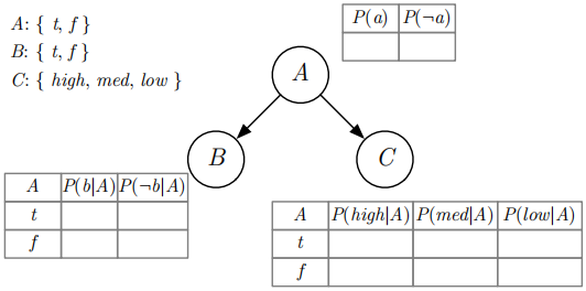
Figure 1: Example of a small Bayesian network possibly useful during development
We said earlier that for finite domains like we are considering, a prior (or unconditional) probability distribution is a mapping from the possible values of a variable to the prob-ability that the variable has that value. So a mapping. . . could be something involving a hashtable, right? But also consider that the domains are generally not very large, so maybe a simple array or list of value-probability pairs would be easier and perhaps even faster in practice.
For finite domains, a posterior (or conditional) probability distribution is a table (a condi-tional probability table, or CPT). Each CPT is “for” the variable at that node. Each row of the table corresponds to an assignment of values to its parents’ variables. The columns of a CPT give the probabilities for each value of the variable, given the assignment for the row. So the table can be thought of as a mapping from assignments to distributions, although that might not be the easiest way to implement them.
One warning for Java programmers: hashtables whose keys are not instances of builtin classes can be tricky. Be sure you understand how hashCode and equals work (see the documentation for java.lang.Object for a discussion).
So now you’ve got the basic framework of classes setup. You should be able to create a small Bayesian network in code, perhaps like the one shown in Figure 1. You could also create the Burglary/Earthquake Alarm network (AIMA Figure 14.2) and the Wet Grass example (AIMA Figure 14.12) by hand if you want.
Time to think about inference. And then you still need to tackle the problem of reading networks from files.
Exact Inference
For the first part of the project, you must implement the “inference by enumeration” algorithm described in AIMA Section 14.4. Pseudo-code for the algorithm is given in Figure 14.9. Section 14.4.2 suggests some speedups for you to consider.
You should be able to turn the pseudo-code into real code using your classes and inter-faces (or whatever you Java haters are doing). I actually copy the pseudo-code into my code file, put “//” in front of it to make it into comments, and use it as a guide as I write the code.
One comment from hard experience: The inference by enumeration algorithm requires that the variables be set in topological order (so that by the time you need to lookup a probability in a variable’s node’s conditional probability table, you have the values of its parents). I don’t think that the pseudo-code in the textbook makes this clear.
You should be able to have your implementation answer queries on the small network that you built by hand. You can compute the correct answers by hand for any choice of probabilities in the network. You could also test your implementation on the Alarm and Wet Grass networks if you created them, since there are exact answers for one query for each of them in the book (and you could work out more by hand).
Approximate Inference
You need to implement algorithms for approximate inference in Bayesian networks. The algorithms described in the textbook and in class are:
1. Rejection sampling
2. Likelihood weighting
3. Gibbs sampling
The first two are straightforward to implement once you have the representation of Bayesian networks and their components, but they can be very inefficient. Gibbs sam-pling is not that hard, although the part explained at the bottom of AIMA page 538 is a bit complicated. One warning: Gibbs sampling may require a large number of samples (look into the issue of “burn-in” in stochastic algorithms).
You must implement the first two algorithms. You may implement Gibbs Sampling for extra credit up to 20%.
Gibbs Sampling, should you choose to implement it, is a bit more complicated than the other two approximate inference algorithms for Bayesian networks. The main challenge is the step in the AIMA Fig 14.16 pseudo-code that says to sample from the distribution P(Zi|mb(Zi)) where “mb” means “Markov blanket.”
AIMA p. 538 under “Why Gibbs Sampling Works” says that, in principle, each variable is sampled conditionally on the current values of all the other variables. You could do that with any inference method for Bayesian networks. However they then say that, for Bayesian networks, sampling conditionally on all variables is equivalent to sampling conditionally on the variable’s Markov blanket. They refer you to p. 517, after which Fig 14.4 shows that the Markov blanket of a variable is its parents, its children, and its children’s parents. And Exercise 14.7 asks you to prove the independence property.
Long story short: Eq. 14.12 at the bottom of p. 538 gives you a formula for computing P(xi|mb(Xi)) using only a few of the probabilities in the network. You don’t need to run a full inference computation, which is good because you have to do this sampling-given-the-Markov-blanket thing at every step of the Gibbs sampling process.
Reading Bayesian Networks From Files
Creating Bayesian networks by hand using code is incredibly tedious and error-prone. So for full points, you need to be able to read in networks from files. This is also the only way that we can test you program, since we aren’t going to a bunch of programming to setup a new problem.
We will give you Java code for parsers that read two quasi-standard file representa-tions for Bayesian networks: the original BIF format (Cozman, 1996) and its successor XMLBIF (Cozman, 1998). The download for this project contains several example net-works (see below for descriptions), and there are many others available on the Internet.
If you develop your own representation classes, which I highly recommend, you should definitely be able to use the XMLBIF parser with a little reverse-engineering. The BIF parser might be harder, since it was itself generated from a grammar of the BIF format using ANTLR.
Whatever you do, you must be able to read XMLBIF files and should be able to read BIF files. Explain in your README which formats your programs can handle.
Running Your Programs
Your implementation must be able to handle different problems and queries. For exact inference, your program must accept the following arguments on the command-line:
• The filename of the XMLBIF encoding of the Bayesian network.
• The name of the query variable, matching one of the variables defined in the file.
• The names and values of evidence variables, again using names and domain val-ues as defined in the file.
So for example, if this was a Java program, you might have the following to invoke it on the alarm example:
java -cp "./bin" MyBNInferencer aima-alarm.xml B J true M true
That is, load the network from the XMLBIF file aima-alarm.xml, the query variable is B, and the evidence variables are J with value true and M also with value true.
The “wet grass” example from the book (also included with my code) might be:
java -cp "./bin" MyBNInferencer aima-wet-grass.xml R S true
The network is in XMLBIF file aima-wet-grass.xml, the query variable is R (for Rain) and the evidence is that S (Sprinkler ) has value true.
The output of your program must be the posterior distribution of the query variable given the evidence. That is, print out the probability of each possible value of the query variable given the evidence.
Your README must make it very clear how to run your program and specify these parameters. If you cannot make them work as described above, you should check with the TAs before the deadline. You can also use make or similar tools for running your programs from the comamnd-line.
If you are using Eclipse and cannot for some reason also make the programs run from the command-line, you MUST setup Eclipse “run configurations” to run your classes with appropriate arguments, and document their use in your README.
For running approximate inferencers, you need to specify the number of samples to be used for the approximation. This should be the first parameter to your program. For example:
java -cp "./bin" MyBNApproxInferencer 1000 aima-alarm.xml B J true M true
This specifies 1000 samples be used for the run. The distribution of the random variable B will be printed at the end of the run. If you need additional parameters, document their use carefully in your README.
Bayesian Network Examples
You should test your inference problem solvers on the AIMA Alarm example (Fig. 14.2) and the AIMA Wet Grass example (Fig 14.12). You should try different combinations of query variable and evidence. You can work out the correct answers by hand if necessary. Note that these both use only boolean variables, but in general variables may have any (finite) domain.
Here are a few more examples of Bayesian networks and references to the literature where they were introduced. We may use some of these to test your program (in addition to the AIMA problems), and we may use some that are not listed here.
• The “dog problem” network from (Charkiak, 1991).
• The “car starts” problem from (Heckerman, at al, 1995).
• The SACHS protein-signaling network from (Sachs et al., 2005).
• The ALARM network for determing whether to trigger an alarm in a patient moni-toring system, from (Beinlich et al., 1989).
• The INSURANCE network from (Binder et. al, 1997).
• The HAILFINDER network from (Abramson et al., 1996).
Most of these are available in one of the code bundles available for this project.
Code Resources
You should try to write the code for this project yourself.
TRY IT. YOU WILL LEARN THE MOST IF YOU DO THIS YOURSELF.
If you give it a solid try and just can’t get it right, we have provided some resources for you:
• You may download the javadoc documentation for my implementation of the project. This includes the abstract specification (package bn.core) and the documenta-tion for all the classes including the inference algorithms (package bn.inference). But I strongly urge you to do it yourself before you look at mine. File: CSC242-project-03-doc.zip
• If you really can’t write the abstract specifications, you may download mine. File: CSC242-project-03-core.zip
• If you really can’t implement the data structures, you may download mine (pack-ages bn.base and bn.util). File: CSC242-project-03-base.zip
• You may download the code for the BIF and XMLBIF parsers, for use with your own code or with mine, as described above (package bn.parser). File: CSC242-project-03-parser.zip
• You may download the set of examples, including examples of creating Bayesian networks manually for the AIMA burglary and wet grass examples (package bn.examples). File: CSC242-project-03-examples.zip
You must still implement the inference algorithms by yourself. So not only will you learn more by doing the rest yourself also, it is often the case that it’s harder to figure out somebody else’s code than designing and writing your own.
I strongly suggest that you avoid the “Java Bayes” website for the duration of this project.
Project Submission
Your project submission MUST include the following:
1. A README.txt file or PDF document describing:
(a) Any collaborators (see below)
(b) How to build your project
(c) How to run your project’s program(s) to demonstrate that it/they meet the requirements
2. All source code for your project. Eclipse projects must include the project set-tings from the project folder. Non Eclipse projects must include a Makefile or shell script that will build the program per your instructions, or at least have those instructions in your README.txt.
3. A completed copy of the submission form posted with the project description. Projects without this will receive a grade of 0. If you cannot complete and save a PDF form, submit a text file containing the questions and your (brief) answers.
Writeups other than the instructions in your README and your completed submission form are not required.
We must be able to cut-and-paste from your documentation in order to build and run your code. The easier you make this for us, the better grade your will be. It is your job to make both the building and the running of programs easy and informative for your users.
Programming Practice
Use good object-oriented design. No giant main methods or other unstructured chunks of code. Comment your code liberally and clearly.
You may use Java, Python, or C/C++ for this project. I recommend that you use Java. Any sample code we distribute will be in Java. Other languages (Haskell, Clojure, Lisp, etc.) by arrangement with the TAs only.
You may not use any non-standard libraries. Python users: that includes things like NumPy. Write your own code—you’ll learn more that way.
If you use Eclipse, make it clear how to run your program(s). Setup Build and Run config-urations as necessary to make this easy for us. Eclipse projects with poor configuration or inadequate instructions will receive a poor grade.
Python projects must use Python 3 (recent version, like 3.7.x). Mac users should note that Apple ships version 2.7 with their machines so you will need to do something differ-ent.
If you are using C or C++, you should use reasonable “object-oriented” design not a mish-mash of giant functions. If you need a refresher on this, check out the C for Java Programmers guide and tutorial. You must use “-std=c99 -Wall -Werror” and have a clean report from valgrind. Projects that do not follow both of these guidelines will receive a poor grade.
Late Policy
Late projects will not be accepted. Submit what you have by the deadline. If there are extenuating circumstances, submit what you have before the deadline and then explain yourself via email.
If you have a medical excuse (see the course syllabus), submit what you have and explain yourself as soon as you are able.
Collaboration Policy
You will get the most out of this project if you write the code yourself.
That said, collaboration on the coding portion of projects is permitted, subject to the following requirements:
• Groups of no more than 3 students, all currently taking CSC242.
• You must be able to explain anything you or your group submit, IN PERSON AT ANY TIME, at the instructor’s or TA’s discretion.
• One member of the group should submit code on the group’s behalf in addition to their writeup. Other group members should submit only a README indicating who their collaborators are.
• All members of a collaborative group will get the same grade on the project.
Academic Honesty
Do not copy code from other students or from the Internet.
Avoid Github and StackOverflow completely for the duration of this course.
There is code out there for all these projects. You know it. We know it.
Posting homework and project solutions to public repositories on sites like GitHub is a vi-olation of the University’s Academic Honesty Policy, Section V.B.2 “Giving Unauthorized Aid.” Honestly, no prospective employer wants to see your coursework. Make a great project outside of class and share that instead to show off your chops.
References
Abramson, B., J. Brown, W. Edwards, A. Murphy, and R. L. Winkler (1996). Hailfinder: A Bayesian system for forecasting severe weather. International Journal of Forecasting, 12(1):57-71.
Andreassen, S., R. Hovorka, J. Benn, K. G. Olesen, and E. R. Carson (1991). A Model-based Approach to Insulin Adjustment. In Proceedings of the 3rd Conference on Artificial Intelligence in Medicine, pp. 239-248. Springer-Verlag.
Beinlich I., Suermondt H.J., Chavez R.M., Cooper G.F. (1989). The ALARM Monitoring System: A Case Study with Two Probabilistic Inference Techniques for Belief Networks. Proceedings of the 2nd European Conference on Artificial Intelligence in Medicine, pp. 247–256.
Binder, J., D. Koller, S. Russell, and K. Kanazawa (1997). Adaptive Probabilistic Net-works with Hidden Variables. Machine Learning, 29(2-3):213–244.
Charniak, E. (1991). Bayesian Networks Without Tears. AI Magazine, Winter 1991, pp. 50–63.
Cozman, F. (1996). The Interchange Format for Bayesian Networks [BIF]. Website at http://sites.poli.usp.br/p/fabio.cozman/Research/InterchangeFormat/xmlbif02.html (accessed March 2019).
Cozman, F. (1998). The Interchange Format for Bayesian Networks [XMLBIF]. Website at http://sites.poli.usp.br/p/fabio.cozman/Research/InterchangeFormat/index.html (accessed March 2019).
Heckerman, D., J. S. Breese, K. Rommelse (1995). Decision-Theoretic Troubleshooting. In Communications of the ACM, 38:49-57.
Sachs, K., O. Perez, D. Pe’er, D. A. Lauffenburger and G. P. Nolan (2005). Causal Protein-Signaling Networks Derived from Multiparameter Single-Cell Data. Science, 308:523-529.
2021-03-28