ACS6116 Advanced Control: Assignment

Dr P. Trodden

Spring 2020–21

Assignment weighting

25% of the total mark for ACS6116

Assignment released

Friday 19th March 2021 (Week 6)

Assignment due

23:59 on Monday 3rd May 2021 (Week 10)

Penalties for late submission

Late submissions will incur the usual penalties of a 5% reduction in the mark for every working day (or part thereof) that the assignment is late and a mark of zero for submission more than 5 working days late. For more information see http://www.shef.ac.uk/ssid/exams/policies.

Feedback

This will include the overall mark, individual component marks and comments on performance on the assignment. The attached assessment criteria (at the back of this document) provides a guide to what areas the feedback will be provided on. Note that marks may be subject to change as a result of unfair means.

Unfair means

The assignment should be completed individually. You should not work together to complete the assignment—it must be wholly your own work. References must be provided to any other work that is used as part of this assignment. Any suspicions of the use of unfair means will be investigated and may lead to penalties. See http://www.shef.ac.uk/ssid/exams/plagiarism for more information.

Exenuating circumstances

If you have extenuating circumstances that cause you to be unable to submit this assign-ment on time or that may have affected your performance, please complete and submit a special circumstances form along with documentary evidence of the circumstances. See http://www.sheffield.ac.uk/ssid/forms/circs, particularly noting point 6 (Medical Circumstances affecting Examinations/Assessment).

Assignment briefifing

This laboratory assignment will assess your fundamental understanding of model predictive control and your ability to design MPC controllers and simulate and analyse MPC-controlled systems.

    The assignment comprises an open-ended design and/or analysis exercise: you are asked to choose one of the listed topics, and tackle the described problem. Each problem includes elements of design, simulation, and analysis.

    Produce a report (limit: 3 pages in the provided template) containing your an-swer.

    In order to create a level playing field between candidates’ submissions, you are asked to prepare your submission using the document templates supplied on Blackboard. This is a 10pt, two-column format, which allows ample space for this assignment even with the 3-page limit. (Please note that no appendices are necessary and even though you may wish to include them, they will not be read.)

    It is up to you how you tackle the problem and stucture your answer. However, it is suggested that you look at (i) the help below and (ii) the attached assessment criteria (at the back of this document) for guidance on what to include.

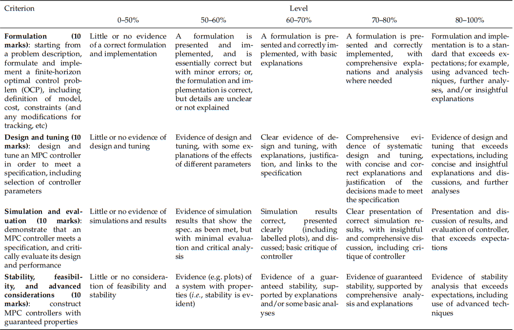
Assessment criteria

The assessment criteria for this exercise are derived from the module learning outcomes, which are:

1. Describe and explain the principles of more than one advanced control technique.

2. Analyse practical performance specifications and convert these into functional requirements on controllers.

3. Design, implement and evaluate an advanced control system against these require-ments.

4. Compare and contrast different advanced control solutions to a particular control problem or application.

5. Describe the receding-horizon principle, and hence compare and contrast LQ-optimal control and MPC.

6. Construct a constrained finite-horizon optimal control problem — including con-straint, model and cost definition — re-formulate it as an optimization problem, and recall and evaluate the analytical expression for the control law in the uncon-strained case.

7. Analyse, design, implement and simulate MPC controllers with guaranteed prop-erties, including feasibility, stability and offset-free tracking.

    In particular, learning outcomes 2, 3, 6 and 7 are relevant to this assessment, and the attached assessment criteria — the marksheet that will be used to assess the assignment

— are derived from these. The marksheet indicates the criteria that will be used in assessing your answer, and also the expectation for each criterion in order to achieve a mark within the specified ranges. It is suggested that you study this marksheet before completing the assignment.

    These assessment criteria are deliberately broad, in order to accommodate the three quite different topics available. Some topics may require more emphasis on certain criteria than others; however, no student will be disadvantaged by topic choice.

    Please note that a 3-page limit, using the supplied template, applies to your report, and you should consider carefully how you can effectively meet the assessment criteria within this limit.

Guidance

• This assignment briefing, lecture slides, and the laboratory exercise document provide the main information that is required to complete this assignment. You may wish, however, to consult the literature relevant to your problem (especially for Topics 2 and 3) and review it in your report.

• Basic MATLAB programming is required, including the use of functions and loops; however, in tackling the assignment you may use the MPC-specific MATLAB functions (used in the laboratory exercises) available on the Blackboard page for ACS6116, plus any code you have developed to answer the laboratory exercises.

• The non-assessed exercises which you completed in the laboratory are good preparation for this assignment. However, the laboratory exercises were well structured, whereas this assignment is open-ended: you need to decide what is the most appropriate approach to solve this assignment, and also how to present your results.

• Regarding the report, you are recommended to consult the attached assessment criteria for guidance on what to include and to what level of detail. In particular, the assessment criteria suggest that your report might need to include, among other things,

– Details of the optimal control problem / MPC formulation you used, includ-ing the correct identification and implementation of constraints.

– A description and explanation of how the controller was designed and tuned in order to meet the specification, including the selection of all parameters, with correct explanations and justifications.

– Clear reporting and discussion of results (including clear, labelled plots), and critical evaluation of the controller. (Think about more than just, for example, “Did my controller meet the spec.?” — what are the strengths and weaknesses of your solution? What could be improved?)

– Some analysis, evaluation and/or qualification of stability and feasibility — does your design come with stability and feasibility guarantees? If so, what are these, and how are they achieved? What else can you say or show? 

This is not an exhaustive list, and what you should include will vary depending on the topic you choose. However, a suggested outline for any report is

1. Abstract

2. Introduction

3. Problem statement

4. Design

5. Results

6. Analysis and discussion

7. Conclusion

This might not be the ideal structure for your report, however, and you may wish to combine or change some of these sections, depending on the topic you choose and the progress you make.

You do not need to include the code that you write, but you may do so (e.g. snippets of code) if you think it adds particular value to your report.

Please note that, in order to achieve the very highest marks, you will need to go beyond simply implementing the methods that you have learned in the lectures and practised in the lab. Surprise me.

• If you do not manage to achieve a working controller or simulation, simplify things, get something simpler working, and build systematically towards a com-prehensive solution. In fact, I advise in all cases to start tackling the problem without constraints, in order that you can get something working without having to wrestle with infeasibility and instability issues (which often arise from incorrect implementation of constraints).

• Should you need clarification or have questions on any part of the assignment then please just ask! (Talk to me in the synchronous sessions, post to the discussion board, or email me at p.trodden@shef.ac.uk).

Submit your report via Blackboard by 23:59 on Monday 3rd May 2021

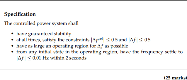
Topic 1: Frequency control in a power system

The operation of an isolated power system under primary frequency control is modelled by the following block diagram.

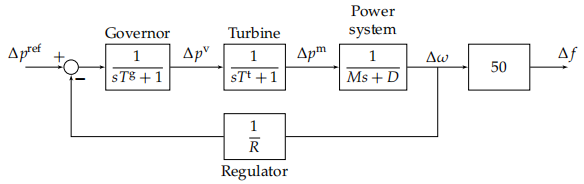
    A steam turbine produces mechanical power, pm, which is subsequently converted to electrical power at a nominal frequency ( = 50 Hz) via a synchronous generator connected to the grid. Changes in power demand (from consumers/loads) and other uncertainties cause deviations in frequency, ∆f = f − . The control objective is to maintain these frequency deviations, ∆f , close to zero. To aid this, a governor controls the steam flow input to the turbine in response to the error between the reference power ∆p^ref and the regulated frequency deviation ∆w/R, where R > 0 is the regulation factor.

    The primary frequency control loop present in the system does not, unfortunately, offer adequate control. Therefore, the aim is to design a secondary frequency control loop that will adjust the reference power ∆p^ref in response to frequency deviations in order to improve transient performance. To this end, a continuous-time state-space model of the system is given as:

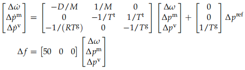
In this model, the input, u = ∆p^ref, is the change in reference power to the turbine governor (in per unit (p.u.) – that is, normalized with respect to a base value of power), and the output, y = ∆f , is the frequency deviation (Hz). The states are the (deviations from operating points in) angular frequency, ∆w, mechanical output power of the steam turbine, ∆p^m, and output power reference from the turbine governor, ∆p^v . For the particular power system under consideration, the model parameters are

    Your task is to design, implement and tune an MPC controller for this system in order to meet the specification on the following page. You may assume that the full state is measurable at each sampling instance. To obtain the discrete-time prediction model for controller, use a sampling time of 0.1 seconds and zero-order hold sampling (i.e. sysd = c2d(sysc,0.1) in MATLAB). When simulating your controller, you may assume that the discrete-time model is an accurate representation of the plant; you do not need to simulate the effect of a sampled-data MPC controller on a continuous-time plant.

Topic 2: Rocket landing control

The SpaceX company achieved the first successful propulsive vertical landing of an orbital-class rocket stage in December 2015¹ . The rocket in question, Falcon 9, is equipped with Merlin 1D rocket engines, capable of vectored thrust, and grid fins which deploy from the stage-1 fuselage following separation; these actuators allow sufficient control-lability of the rocket to permit a safe vertical landing. From a technical point of view, the successful landings were also enabled by theoretical advances in how the kind of nonlinear optimal control problem associated with safe rocket landing can be modelled and solved².

    A simplified model of the rocket landing problem—assuming that “nose-up” stabi-lization is handled separately—views the rocket as a point mass, m, with position 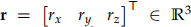 and velocity . The coordinates  are defined with z measured vertically upwards from ground (so z = 0 is sea level) and so that (x, y) is the lateral plane parallel to ground. The net thrust vector emerging from the engine is 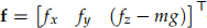—where the z component is explicitly accounting for gravity—which causes acceleration of the mass according to the (discretized) dynamics

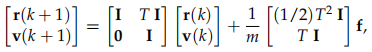
where I is the 3 × 3 identity matrix, 0 is the 3 × 3 matrix of zeros, and T is the sampling time, which you may assume to be 0.5 s.

    The aim is to steer the rocket from an initial position r(0) and velocity v(0) to the target ground position rt = 0 at rest (vt = 0). This should be done safely and at minimum fuel cost; that is, a number of constraints should be met during the mission:

• The engines are capable of exerting a thrust satisfying:

– limits on vertical thrust: .

– limits on lateral thrust:

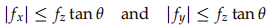
where θ = 10 degrees is the maximum angle for thrust vectoring.

• The vertical speed shall not exceed 15 m s^-1 in descent.

• The lateral speeds, |vx| and |vy|, shall not exceed 20 m s^-1.

• In order to avoid premature ground collision, the positional trajectory shall respect a glide-slope constraint

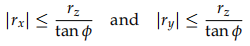
where is the glide-slope angle, and is 30 degrees.

    Your task is to design, implement and tune an MPC controller for this system in order to achieve safe landing from initial altitudes up to 500 m and initial lateral distances up to 600 m from the target. You should investigate the feasibility of the mission for a range of different initial positions and also non-zero initial velocities, representing the real situation of the rocket already having downward and lateral speed at the commencement of landing control. You might wish to consider that, although it is desired to minimize fuel, the landing should complete in finite (as opposed to infinite) time.  

(25 marks)

Topic 3: State constraints and stability

In a seminal 1993 paper by Kenneth Muske and James Rawlings³ , it was shown that the following system

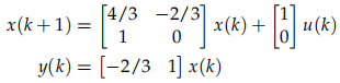
is difficult to stabilize in the presence of a simple constraint on the output y(k).

    Your task is to conduct a rigorous investigation into the stability of this system. The output constraint that should be applied is

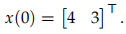
and the desired tuning parameters for the MPC controller are Q = I, R = 1 and N = 5. A problematic initial state in this setting is

A non-exhaustive list of suggestions for what your investigation could include:

• Whether the system can be stabilized, by tuning Q, R and N, without using stabilizing terminal ingredients (i.e., a stabilizing P and/or terminal set).

• Whether the use of stabilizing terminal ingredients can stabilize the system and, if so, what those terminal ingredients should be.

• How sensitive the problem is to the magnitude of the output constraint; for example, if the limit on y(k) is increased to 1 + e, what value of e is needed to ease the instability problem.

• Exploration of the region of feasibility (set of states for which the problem is feasible) and region of attraction (set of states from which the system may be stabilized).

(25 marks)