High-performance Computing

Coursework Assignment

Deadline: 24th March 2021 - 23:00

1 Introduction

The objective of this coursework is to write a parallel numerical code for solving a two-dimensional smoothed particle hydrodynamic (SPH) formulation of the Navier-Stokes equations. SPH models the behaviour of fluids by approximating the fluid properties using smooth kernel density functions. Each particle therefore only influences neighbouring particles within a given radius and properties of the fluid are smoothed between particles.

The position and velocity of each particle are updated at each time step using an explicit time-integration scheme. We calculate these state variables by updating our approximation to the fluid density, pressure and viscous forces on each particle and use these to calculate the acceleration of the particles.

The equations for SPH are derived from the Navier-Stokes equations. Primarily we need to enforce conservation of linear momentum. The derivation of these equations can be found in textbooks.

Figure 1: Illustrative SPH simulation of a droplet, represented by a collection of particles, hitting a surface.

2 Algorithm

The simulation consists of a set, P, of N particles, with positions xi and velocities vi . Each particle has a mass m and a radius of influence h, beyond which no interaction with other particles is considered. The computational domain is a box Ω = [0, 1]² . The parameters for the problem are:

For a single time-step the algorithm proceeds as follows:

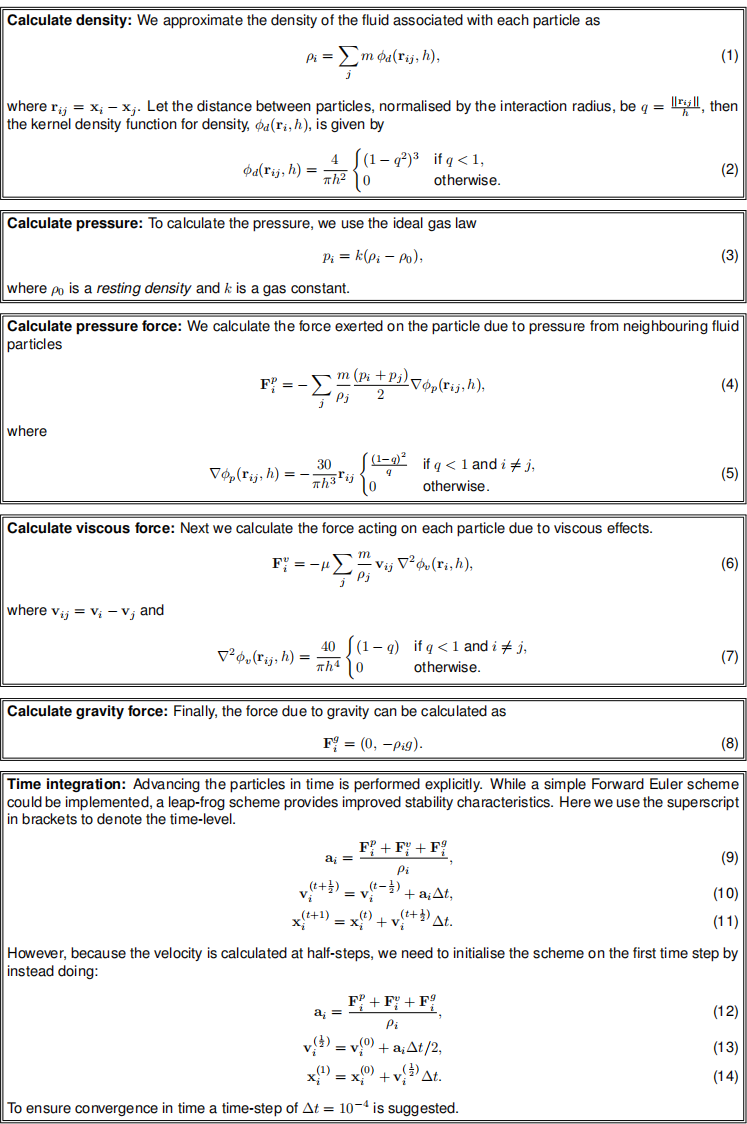
2.1 Initial Condition

To initialise the simulation, one or more particles must be specified. These should be evenly distributed. Some examples are suggested in the test cases.

Once the particles are placed, the particle densities should be evaluated with an assumed mass of m = 1 and the mass subsequently scaled so that the density is equal to the reference density:

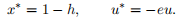
2.2 Boundary Conditions

All the boundaries are solid walls with damped reflecting boundary conditions. If particles are within a distance h of the boundary, their velocity and position should be updated to reverse the motion of the particle and keep it within the domain. For example, on the right boundary, the x-component of position and velocity would be modified as

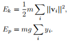
2.3 Energy

The motion of particles within the interior of the domain should be energy conserving. As particles strike the boundaries, their motion is damped and therefore lead to a loss of energy from the system.

The kinetic energy and potential energy of the system can be calculated as:

3 Code Development

3.1 Validation cases

When developing your code, the following test cases may be helpful to assess the correctness of your code:

• A single particle at (0.5, 0.5) to test the correctness of time integration and gravity forcing, as well as the bottom boundary condition.

• Two particles at (0.5, 0.5) and (0.5, h) to assess the pressure force and viscous terms. Try changing µ and k.

• Three particles at (0.5, 0.5), (0.495, h) and (0.505, h) to assess left and right boundary conditions. Try changing e.

• Four particles at: (0.505, 0.5), (0.515, 0.5), (0.51, 0.45) and (0.5, 0.45) to assess multiple particle interaction.

3.2 Test cases

These are more interesting initial conditions and are useful for assessing the performance of your code: 

• Dam break: a grid of particles occupying the region [0, 0.2]2.

• Block drop: a grid of particles occupying the region [0.1, 0.3] × [0.3, 0.6]

• Droplet: particles occupying a circle of radius 0.1, centred at the point [0.5, 0.7].

You may need to add small amplitude noise to the particle positions to see more realistic behaviour.

3.3 Command-line input

Your code should accept the following parameters as command-line arguments (do not prompt the user to enter input during the execution of your program):

--ic-dam-break           Use dam-break initial condition.

--ic-block-drop           Use block-drop initial condition.

--ic-droplet                Use droplet initial condition.

--ic-one-particle         Use one particle validation case initial condition.

--ic-two-particles        Use two particles validation case initial condition.

--ic-four-particles       Use four particles validation case initial condition.

--dt arg                     Time-step to use.

--T arg                      Total integration time.

--h arg                      Radius of influence of each particle.

3.4 File output 

Your code should generate a file called output.txt with the position of all particles at the final time, specified as two columns (x- and y-coordinates, separated by space). You may output this file at intermediate times (e.g. every second of simulation time) if you wish.

Your code should also generate a file energy.txt with four columns of data: the time, kinetic energy, potential energy and total energy at each time step.

3.5 Optimisation and Parallelisation

You should undertake some basic performance optimisation of your implementation and parallelise your code using MPI. There are several approaches to parallelisation for this problem. You should discuss in the report the approach you have chosen and why.

Tasks

The objective of this coursework is to write a high-performance parallel, object-oriented, C++ code which will solve the SPH problem as described above. In completing this assignment you should write a single code which satisfies the following requirements:

• Reads the parameters of the problem from the command line (do not prompt the user for input). Please use the exact syntax given for the parameters in section 3.3 as these will be used when testing your code. [5%]

• Implements a class called SPH to solve the SPH problem using the algorithm described above. You are free to add any additional functions and classes, as required. [30%]

• Generates an appropriate initial set of particles based on the command line arguments given. [5%]

• Is parallelised using MPI. It should be able to run on at least two processes (as specified by the -np param-eter to mpiexec). [30%]

• Uses a build system (Make or CMake) to compile your code and uses git for version control. Provide evidence of the latter by running the command

git log --name-status > repository.log

and including the file repository.log in your submission. [5%]

• Uses good coding practices (code layout, comments, documentation) [5%]

• Is accompanied by a report (max 3 pages) as detailed below. [20%]

Report (3 pages)

Write a short and concise report which includes:

• plots of the potential energy, kinetic energy and total energy of the system (all on the same plot) as a function of time, for the three test cases in section 3.2 (three plots in total) until they reach steady state ;

• a discussion of the serial performance of your code, highlighting the parts of your implementation which take the longest and any code optimisations you have applied to improve the execution speed;

• a discussion of how you chose to parallelise your code (and why) as well as any design decisions you explicitly made to enable this.

Submission and Assessment

When submitting your assignment, make sure you include the following:

• All the files needed to compile and run your C++ code:

– Source files for a single C++ program which performs all the requirements. i.e. All .cpp and .h files necessary to compile and run the code.

– The Makefile or CMakeLists.txt file (as preferred) used for compiling your code and linking with any necessary libraries.

• Your three-page report (in PDF format only).

• The git log (repository.log).

These files should be submitted in a single ZIP archive file to Blackboard Learn.

It is your responsibility to ensure all necessary files are submitted.

You may make unlimited submissions and the last submission before the deadline will be assessed.

END OF ASSIGNMENT