Exotic searches at ATLAS with NN Classification
DAML Week 7, CP15:
Exotic searches at ATLAS
with NN Classification
Christos Leonidopoulos∗
University of Edinburgh
March 4, 2021
1 Introduction
In this lecture we are returning to classification problems with Neural Networks (NN). We have seen in the previous Semester how one can use a NN to make a particle identification (e.g. “proton”, “positron” or “pion”, etc.). A very similar problem in particle physics is one in which we are trying to train a NN discriminator to differentiate between signal and background classes of events by using information about the underlying physics contained in kinematic variables, e.g. from particles colliding at an accelerator. This is a binary (and supervised) classification problem, i.e. the classification has only two possible discrete outcomes. Such problems in particle physics tend to be multi-dimensional and non-linear, with the NN requiring a large number of inputs (i.e. the kinematic variables).
In today’s lecture we will be using simulated data from the ATLAS experiment [1] at CERN. We will be deploying NN techniques for classification in a search for exotic par-ticles, and evaluate the performance of these architectures, as we have done before.
2 Search for heavy resonances decaying into vector boson pairs at ATLAS
There are many exotic models that predict new exotic (also known as “Beyond the Stan-dard Model”) particles. Searches for new particles tend to focus on the large-mass region of the phasespace, as the assumption is that lighter particles would have been discovered in searches at previous experiments at lower collision energies.
For today’s problem, we are considering a search for an (additional) heavy Higgs boson decaying into pairs of vector bosons V (where V = W or Z), see Fig. 1. Hadronic decays of vector bosons have large branching fractions but also large backgrounds, whereas leptonic decays come with lower branching fractions and a cleaner experimental signature. A compromise between large backgrounds and very small signal yields is to require one of the vector bosons to be a Z decaying leptonically  , with the second vector boson decaying hadronically
  . One would expect the hadronisation of the two quarks to give two distinct reconstructed jets of particles inside the detector. However, for V bosons originating from very heavy particles (in the TeV region) encountered in typical exotic-search signatures at the Large Hadron Collider (LHC) [2], the quarks from the hadronic V decay tend to partially overlap in the
  space, giving rise to an experimental signature that requires special treatment. Searches that include this boosted, partially-overlapping quark hadronisation use the so-called “fat” (large-R) jet reconstruction (J). The aim is to differentiate this experimental signature from the one of single-quark or gluon hadronisation, typically captured with the baseline jet reconstruction algorithm (j).
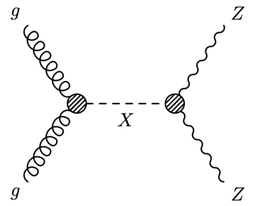
Figure 1: Representative Feynman diagram for the production of a heavy resonance X via gluon fusion (incoming gg pair), with its subsequent decay into a pair of vector bosons (specifically: ZZ in this diagram). In the example of the X decay into a pair of Z bosons, this analysis described in the text would be sensitive in the final state in which one of the Z bosons decays leptonically, with the second one decaying hadronically.
In any physics analysis, one of the most important ingredients is the characterisation of the experimental signature of the final state with a list of decay products. For the search of heavy Higgs bosons, the chosen final state here is two opposite-sign charged leptons ( +−, with = e or µ), and one fat-jet (J). Additional requirements may be that the invariant mass of the charged leptons is consistent with the Z boson mass (
 91 GeV/c2 ), or that the invariant mass of the dilepton pair and the fat jet are consistent with the Higgs boson mass2.
The next task is to identify potential sources of SM background processes that could mimic the signal of interest. The most obvious one is the non-peaking diboson contin-uum, qq → Z( )V (
)V ( ). We should also add the inclusive Z production, qq → Z()+ jets. Finally, we should include the
  production, since the leptonic decays of the W bosons from the t → W b decays can lead to final states with two charged leptons (and occasionally boosted jets).
We will be working with simulated datasets for all these (signal and background) pro-cesses, containing kinematic information for all decay products of interest.
3 Signal and background datasets
CSV files with the kinematic information for about 680k background and 50k signal simu-lated events can be found at https://cernbox.cern.ch/index.php/s/kAqx9oaS716zia53. The background events are split into three different files corresponding to different physics processes. The signal sample has been generated for a hypothetical heavy Higgs boson with  = 1 TeV/c2 . Every entry in these tables corresponds to a separate (signal or background) collision event.
The files contain a large number of variables per event. Here we will focus on a subset of them, summarised in Table 1.
|
Variable
|
Description
|
|
lep1_pt
|
transverse momentum of fifirst reconstructed lepton (in MeV/c)
|
|
lep2_pt
|
transverse momentum of second reconstructed lepton (in MeV/c)
|
|
fatjet_pt
|
transverse momentum of reconstructed fat-jet (in MeV/c)
|
|
fatjet_eta
|
η of reconstructed fat-jet
|
|
fatjet_D2
|
 of reconstructed fat-jet of reconstructed fat-jet
|
|
Zll_mass
|
invariant mass of reconstructed dilepton system (in MeV/c2)
|
|
Zll_pt
|
transverse momentum of reconstructed dilepton system (in MeV/c)
|
|
MET
|
transverse missing energy in reconstructed event (in MeV)
|
|
reco_zv_mass
|
invariant mass of reconstructed dilepton-plus-fatjet (
J) system (in MeV/c2)
|
|
isSignal
|
boolean flag: 0 for background, 1 for signal
|
Table 1: List of subset of kinematic variables contained in CSV files to be used in this analysis, and brief description.
Notes:
•
• Events with one or more neutrinos (e.g.
).
4 Data inspection and variable plotting
We will be using the keras [4] library for today’s classification problem.
We will start with the usual steps of opening the CSV files, inspecting the data in case it requires cleaning, and plotting a few distributions in order to better understand the available handles for differentiating between signal and background.
Exercise #1 (1 point):
Open the three background and one signal CSV files, and feed the data into four pandas.core.frame.DataFrame objects. One of them is significantly larger than others, and it will take much longer to unpack. You may want to use command os.path.getsize as a warning to your reader/self.
Carry out the usual sanity checks (pandas.core.frame.DataFrame.head(5)), and de-termine if data-cleaning is necessary (pandas.core.frame.DataFrame.dropna(inplace = True)).
Plot 1D distributions for the first 9 variables listed in Table 1, with one plot per variable and the distributions categorised by physics process (1 category for signal, 3 categories for background). Make sure the distributions are normalised (i.e. we are interested in shape differences here, not the overall integrated contributions), and that they are clearly distinct for the different processes (e.g. use different colours and non-filled histograms).
You can use a loop over the input features to simplify the code, and you can ignore the units on the x-axis.
5 Classification with Neural Networks
We will initially use as input features the first 8 kinematic variables that appear in Table 1, i.e. we will ignore variable reco_zv_mass for now. The invariant mass of the heavy resonance targeted by a search is traditionally used as the discriminant of choice. Will the decision to ignore it here hurt the sensitivity of the NN? As we will see, including this variable in the input features does make a difference, however maybe not as dramatic as one would expect. However, this is not very surprising, given the rest of the kinematic information that is already fed into the NN.
isSignal is the target variable, i.e. the binary variable whose value we are trying to predict given the set of input features.
Exercise #2 (2 points):
(a) (1 point) Put together all background samples to produce one “mega” DataFrame with method pandas.core.frame.DataFrame.concat. You probably also want to be using the ignore_index=True option.
We want to shuffle the contents of the new DataFrame, as it currently contains or-dered events from different background processes, which is unnatural. Use methods sklearn.utils.shuffle and DataFrame.reset_index(drop=True). Make sure to run this with a fixed random seed, as per good practice for reproducibility of your results.
Create a training dataset that contains equal numbers of signal and background events. Remember that in the original dataframes the number of background events is much larger than the number of signal events. Create a 50-50 admixture sample with twice the number of signal events4 . Use the previously discussed concat and shuffle methods.
(b) (1 point) Create a new dataframe containing only the 8 input and 1 output features of interest. Make 2D scatter plots for each combination pair of the 8 input features. Choose a different colour for signal and background (do this by creating a wtype = [’Background’, ’Signal’] object with the labels of the possible N_classes = 2 cate-gories. You can either write your own code, or recycle function dt_utils.featureplot that we used in a previous NN checkpoint.
Hint: See https://cernbox.cern.ch/index.php/s/z2OTPim0XoXr4dI for some handy utilities that you can use in today’s checkpoint.
We will now start preparing the data before feeding them into the NN. We will standardise the inputs by scaling their ranges so that they are roughly the same. We then create training and test subsets, as usual.
Exercise #3 (1 point):
We start by performing input-feature scaling. We then split the dataset into training (70%) and test (30%) subsets:
from sklearn import model_selection , preprocessing
sc = preprocessing . StandardScaler ()
input_data = sc . fit_transform ( input_data )
# set random seed
Answer_to_all_questions = 42
# train - test split of dataset
train_data , test_data , train_target , test_target = model_selection . train_test_split (\
input_data , target , test_size =0.3 , random_state = Answer_to_all_questions )
print ( train_data . shape , train_target . shape , test_data . shape , test_target . shape )
We will now create a function that can build flexible NNs of varying depth (i.e. number of layers) and width (i.e. number of nodes per layer). We will also make the testing of various architectures easier and faster than previous checkpoints.
We will be using the accuracy of the NN prediction as the metric to identify the most performant architecture.
|
Exercise #4 (3 points): (a) (2 points) Write a function that can create flexible NN models. def my_model ( num_inputs , num_nodes , extra_depth ): # create model model = Sequential () model . add ( Dense ( num_nodes , input_dim = num_inputs , kernel_initializer =’normal ’, \ activation =’relu ’)) model . add ( Dropout (0.2)) for i in range ( extra_depth ): # code up the extra layers here model . add ( Dense ( num_outputs , activation =’sigmoid ’)) # Compile model model . compile ( loss =’ binary_crossentropy ’, optimizer =’adam ’, metrics =[ ’accuracy ’]) return model Try running the NN with a batch size of 500, 50 epochs, 20 nodes per layer, and extra depth = 1 as a starting point. Put the result of the fit method call into a History object: history = model . fit ( train_data , train_target , batch_size = batchSize , epochs = N_epochs , \ verbose =1 , validation_data =( test_data , test_target )) (b) (1 point) When the classification converges, use arrays History.history[’loss’] and History.history[’val_acc’] to plot the evolution of the loss-function (y-axis in log-scale) and the NN accuracy on the validation sample (y-axis in linear-scale) as a func-tion of the epoch. You may use functions nn_utils.lossplot and nn_utils.accplot or write your own. |
|
Exercise #5 (2 points): Having to find the best architecture by varying the numbers of layers and nodes, or the batch size and number of epochs is quite tedious. We will implement a callback hook that can automate the procedure for us, and exit the optimisation when the classification converges: from tensorflow . keras . callbacks import EarlyStopping , ModelCheckpoint callbacks_ = [ # if we don ’t have an increase of the accuracy for 10 epochs , terminate training . EarlyStopping ( verbose = True , patience =10 , monitor =’val_acc ’) , # Always make sure that we ’re saving the model weights with the best accuracy . ModelCheckpoint (’model .h5 ’, monitor =’val_acc ’, verbose =0 , save_best_only = True , mode =’max ’)] history = model . fit ( train_data , train_target , batch_size = batchSize , epochs = N_epochs , \ verbose =1 , validation_data =( test_data , test_target ) , callbacks = callbacks_ ) Try using this new method after you expand the set of input features to also include variable reco_zv_mass. Feel free to experiment with the architecture parameters. The goal is to achieve an accuracy (val_acc) of 95%. Plot the loss-function and NN-accuracy as a function of the epoch for the best classification method. |
|
Exercise #6 (1 point): We will now try to visualise the results of the NN classifier. Use method keras.models.Model.predict to get the predicted categories for test data. Notice that the output is not binary, but corresponds to a probability. Use a simple model (e.g. predicted = (predict_test_target >0.5)) to turn the output into a binary decision. Use sklearn.metrics.confusion_matrix and nn_utils.heatmap to plot the “confusion matrix” on a 2 × 2 grid. A more advanced way of showing the NN classifier performance is by producing a ROC curve. Use sklearn.metrics.roc_curve to get the False Positive Rate (i.e. effectively: background efficiency) and True Positive Rate (i.e. effectively: signal efficiency). Plot the ROC curve. What would you say the optimal performance point is? |
Check out Ref. [5] for a brief discussion on ROC curves.
6 Summary
In today’s lecture we have seen how to use advanced NN classification techniques to differential between signal and backround processes in simulated ATLAS data. One could try to evaluate if the NN techniques explored today improve the sensitivity of a search in a dataset containing a hint of a signal, compared to the invariant mass discriminant technique that we used in the previous Semester.
References
[1] The ATLAS collaboration, https://atlas.cern/
[2] The Large Hadron Collider (LHC) at CERN, https://home.cern/science/accelerators/large-hadron-collider
[3] “Analytic Boosted Boson Discrimination”, A. J. Larkoski, I. Moult and D. Neill, JHEP 05 (2016) 117, arXiv 1507.03018
[4] Keras, Fran¸cois Chollet et al, https://keras.io
[5] https://scikit-learn.org/0.15/auto_examples/plot_roc.html
2021-03-15