Advanced Structural Analysis and Dynamics 5 – ENG5274

Course Work 1 - Euler–Bernoulli Beam Theory

February 10 2021 Andrew McBride

import numpy as np

import matplotlib.pyplot as plt

import math

Overview

In this report, you will develop and validate a ¦nite element code written in Python for solving Euler–Bernoulli beam theory. The code will extend the one you developed for a linear elastic bar in 1D.

The report is to be uploaded to Moodle by 8 March 2020 (by 15:00).

Submission requirements

Report

The main report document should clearly and logically address all the tasks. Marks will be deducted for poor presentation. The report is to be submitted on-line via Moodle - hard-copies will not be marked.

You are to write the report in the Jupyter Notebook format (IPython) using Markdown for the written report. You can use Google Colab, Jupyter Notebook or your favourite IPython ¦le editor.

For more information on Markdown see https://guides.github.com/pdfs/markdown-cheatsheet-online.pdf. You need to submit:

● the main_EB.ipynb containing the write up and code. No other documents will be accepted.

Code

● Your code needs to be commented and documented.

● You must include the validation examples in your submission.

Primary functions

Primary functions to compute the element stiffness matrix  , the element force vector due to distributed loading  and the local to global degree of freedom map.

def get_Ke(le, EIe):

  '''Return element stiffness matrix

    Parameters

    ----------

    le : double

      Length of element

    EIe : double

      Product of Young's modulus and moment of inertia

  '''

  return

def get_fe_omega(le, fe):

  '''Return force vector due to distributed loading

    Parameters

    ----------

    le : double

      Length of element

    fe : double

      Average distributed load on element

  '''

  return

def get_dof_index(e):

  '''Return the global dof associated with an element

    Parameters

    ----------

    e : int

      Element ID

  '''

  return

Validation problems

Consider a 12 m beam with EI = 1e4 Nm. Ensure that your code is indeed producing the correct results by comparing the computed deflection and possibly rotation with the analytical solution for the following loading conditions:

1. An end-loaded cantilever beam with point load of P = -10 N acting at x = 12 m. The beam is fully fixed at x = 0. Compare the computed tip deflection and rotation with the analytical solution.

2. A cantilever beam with a distributed load of f = -1 N/m acting over the length of the beam. The beam is fully fixed at x = 0. Compare the computed tip de§ection and rotation with the analytical solution.

3. An off-center-loaded simple beam with a point load of P = -10 N acting at m. Deflections are 0 at x = 0 and x = L. Ensure that the load acts at a node. You only need to compare your solution to the analytical solution for the position of, and deflection at, the point of maximum displacement.

4. A uniformly-loaded simple beam with a distributed load of f = -1 N/m acting over the length of the beam. Deflections are 0 at x = 0 and x = L. You only need to compare thedeflection along the length of the beam to the  analytical solution.

Where possible, you should test your code for one element and for multiple elements.

Consult https://en.wikipedia.org/wiki/Deflection_(engineering) for analytical solutions and descriptions of the loading.

Validation - Cantilever with point load

# properties of EB theory

dof_per_node = 2

# domain data

L = 12.

# material and load data

P = -10. 

P_x = L

f_e = 0.

EI = 1e4

# mesh data

n_el = 1

n_np = n_el + 1

n_dof = n_np * dof_per_node

x = np.linspace(0, L, n_np)

le = L / n_el 

K = np.zeros((n_dof, n_dof))

f = np.zeros((n_dof, 1))

for ee in range(n_el):

    dof_index = get_dof_index(ee)

    K[np.ix_(dof_index, dof_index)] +=  get_Ke(le, EI)

    f[np.ix_(dof_index)] += get_fe_omega(le, f_e)

node_P = np.where(x == P_x)[0][0]

f[2*node_P] += P

free_dof = np.arange(2,n_dof)

K_free = K[np.ix_(free_dof, free_dof)]

f_free = f[np.ix_(free_dof)]

# solve the linear system

w_free = np.linalg.solve(K_free,f_free)

w = np.zeros((n_dof, 1))

w[2:] = w free[

]

_

# reaction force

rw = K[0,:].dot(w) - f[0]

rtheta = K[1,:].dot(w) - f[1]

# analytical solution

w_analytical = (P * L**3) / (3*EI)

theta_analytical = (P * L**2) / (2*EI)

print('Validation: cantilever with tip load')

print('------------------------------------')

print('Reaction force: ', rw, '\t Reaction moment: ', rtheta)

print('Computed tip deflection: ', w[-2], '\t Analytical tip deflection: ', w_analy

print('Computed tip rotation: ', w[-1], '\t Analytical tip rotation: ', theta_analy

plt.plot(x,w[0::2],'k-*')

plt.xlabel('position (x)')

plt.ylabel('deflection (w)')

plt.show()

plt.plot(x,w[1::2],'k-*')

plt.xlabel('position (x)')

plt.ylabel('rotation (w)')

plt.show()

Validation - Cantilever with distributed load

# material and load data

P = 0. 

f_e = -1.

# mesh data

n_el = 10

n_np = n_el + 1

n_dof = n_np * dof_per_node

x = np.linspace(0, L, n_np)

le = L / n_el 

K = np.zeros((n_dof, n_dof))

f = np.zeros((n_dof, 1))

for ee in range(n_el):

    dof_index = get_dof_index(ee)

    K[np.ix_(dof_index, dof_index)] +=  get_Ke(le, EI)

    f[np.ix_(dof_index)] += get_fe_omega(le, f_e)

free_dof = np.arange(2,n_dof)

K_free = K[np.ix_(free_dof, free_dof)]

f_free = f[np.ix_(free_dof)]

# solve the linear system

w_free = np.linalg.solve(K_free,f_free)

w = np.zeros((n_dof, 1))

w[2:] = w_free

# reaction force

rw = K[0,:].dot(w) - f[0]

rtheta = K[1,:].dot(w) - f[1]

# analytical solution

w_analytical = (f_e * L**4) / (8*EI)

theta_analytical = (f_e * L**3) / (6*EI)

print('Validation: cantilever with uniformly distributed load')

print('------------------------------------------------------')

print('Reaction force: ', rw, '\t Reaction moment: ', rtheta)

print('Computed tip deflection: ', w[-2], '\t Analytical tip deflection: ', w_analy

print('Computed tip rotation: ', w[-1], '\t Analytical tip rotation: ', theta_analy

plt.plot(x,w[0::2],'k-*')

plt.xlabel('position (x)')

plt.ylabel('deflection (w)')

plt.show()

plt.plot(x,w[1::2],'k-*')

plt.xlabel('position (x)')

plt.ylabel('rotation (w)')

plt.show()

Validation - Off-center-loaded simple beam

# material and load data

Validation - Simple beam with distributed loading

# material and load data

P = 0. 

P_x = 3.

f_e = -1.

EI = 1e4

Problem A: Beam structure with linear loading

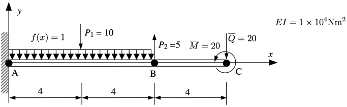
Now consider the L = 12 m beam shown below. The beam is fully ¦xed at point A (x = 0). A distributed load of f(x) = -1 N/m acts between points A and B. Point loads P1 = -10 N and P2 = 5 N act at x = 4 m and x = 8 m, respectively. Natural boundary conditions are comprised of a traction 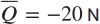and a moment Nm both acting at point C (x = L). The product E1 = 1e4 Nm².

Assumptions

The code you develop for this problem should assume that the number of elements is a multiple of 3. This will ensure that the point loads are applied directly at a node (why is this important?).

Outputs

Use your validated code to:

● Determine the reaction force and moment at point A (for 12 elements). Use these to confirm that your output is correct.

● Plot the deflection over the length of the beam (for 12 elements).

● Plot the rotation over the length of the beam (for 12 elements).

● Plot the bending moment M over the length of the beam (for 12 elements).

Problem B: Beam structure with nonlinear loading

Problem B is identical to that considered in Problem A but the distributed load is given by

Furthermore, the material properties are no longer constant and

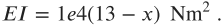
For meshes of 3, 3², 3³, 3⁴ elements, generate plots of

● deflection (at x = 4 m) versus the number of degrees of freedom.

●  versus the number of degrees of freedom.

Explain the method you have used to perform the numerical integration - provide a validation example that shows your method works.

Comment on the convergence of the solution.