MSCI512: Simulation and Stochastic Modelling

2020/21 Coursework Task

Task instructions (please read carefully)

• Please answer any TWO questions out of three.

• The maximum score is 100.

• If you answer all three questions, all three of your answers will be marked and your highest two scores will be counted.

• You are expected to use appropriate software (e.g. Microsoft Excel, R, Python) to help you answer the questions.

• This coursework is related to the Stochastic Modelling part of the module. No credit will be given for using simulation methods to answer the questions. In particular, you should not need to use random number generation in any of your answers.

• Write all non-exact numerical answers correct to at least 3 significant figures. Also, when using non-exact numbers obtained from a previous calculation, make sure these numbers are correct to at least 3 significant figures.

• This coursework is to be done as an individual piece of work. Collusion between students and plagiarism are regarded as serious offences and will be penalised severely. Information about the university’s plagiarism framework can be found here: https://modules.lancaster.ac.uk/mod/resource/view.php?id=1384800.

Submission instructions

• The deadline for submission is 10:00AM on April 12th 2021.

• Your answers to the questions can be either typed (e.g. using Microsoft Word) or handwritten and scanned.

• You should include full details of your methods in your answers. If you calculate answers by hand, you should include all of your calculation steps. If you use computer software (e.g. spreadsheets, computer programs) you should include the relevant files (e.g. .xlsx, .py, .txt) in your submission. Please also include enough explanation in your answers to make it clear what you are doing and why.

Question 1 (50 marks)

A technology company operates several large warehouses which are staffed mainly by robots. These robots perform various essential functions, including picking up packages and transporting them to where they are needed. In order for warehouse operations to run efficiently, it is imperative that robots are kept in good working condition. The company’s engineers use a numerical classification scheme to record the condition of an individual robot, based on the conditions of its essential components, as follows:

4 – Excellent; all components appear to be in perfect working order.

3 – Some components are showing some ‘wear’ and this may be affecting movement speed and/or other functions.

2 – Significant evidence of degradation affecting various functions.

1 – Some components no longer fit for purpose; robot is close to failure.

0 – Failure; robot must be repaired before resuming operations.

Robots’ conditions are inspected at the beginning of every working day. If a robot is in the “failure” state at the beginning of a particular day, it undergoes repairs and this process takes one full day. It then returns to state 4 at the beginning of the next day.

The company would like to understand more about how robots change condition over time, so that they can make better decisions about how to manage their workforce. On October 1st 2020, they launched an experiment in one of their warehouses which worked as follows: the conditions of all robots in the warehouse were examined and 20 robots in “excellent” condition (i.e. state 4) were selected. Each of these robots was monitored at the beginning of every day until it eventually failed (i.e. reached state 0). Robots were no longer monitored after their first failure. The day-by-day results from the monitoring process are shown in the spreadsheet Q1_data.xslx. Note that “Day 1” is October 1st, and the dataset shows results until Day 82, by which time all 20 robots had failed at least once.

Note: The dataset shows that, on rare occasions, the condition of a robot might improve from one day to the next. This can happen if the warehouse’s on-the-floor attendants manage to spot a small ‘glitch’ which is easy to fix.

(a) Use the data provided in the spreadsheet Q1_data.xslx to formulate a Markov chain model of how robots change their condition over time. You should clearly describe the state space of the Markov chain and also provide the transition probability matrix (with transition probabilities estimated from the data). Also discuss the assumptions required in order for the Markov chain model to be considered a valid model of the real-world process. [10 marks]

(b) The warehouse that took part in the experiment currently has 80 robots on duty. As mentioned above, robots in state 0 at the start of a day undergo a repair process and return to state 4 on the next day. The cost of repairs is £200 per robot. Use this information to calculate the average repair cost per day that the company incurs for robots in the warehouse over a large number of days. [5 marks]

(c) Given that a particular robot is in state 2 on October 1st, calculate the probability that it does not fail at any time within the next 10 working days. [5 marks]

(d) The company is interested to know whether it would be more profitable to change their policy for carrying out repairs, so that robots are sometimes repaired even if they have not yet reached the “failure” state. The robots’ conditions (and associated decisions about whether or not they should be repaired) can affect the company’s profits in three different ways, described below:

• Repair cost: As stated in part (b), the repair cost is £200 per robot. However, you should now assume that robots can be repaired even if they are not yet in state 0. Decisions about whether to repair a robot are always made at the beginning of a working day and, after being repaired, a robot is restored to state 4 at the beginning of the next day. The repair cost is mainly a labour cost, and does not depend on the robot’s current condition.

• Productivity cost: When a robot is in a suboptimal condition, the productivity of the warehouse is affected and the company loses money. Estimates of the average daily costs (due to loss of productivity) associated with the different possible robot conditions are shown in Table 1 below.

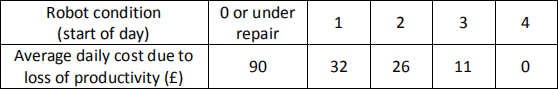
Table 1: Average daily costs due to loss of productivity for different robot conditions

• Reduction in trade-in value: The company may decide to sell some of its robots for cash, but the trade-in value for an individual robot depends on its condition. Table 2 shows the reduction in the sale price for the various different robot conditions. For example, a robot in state 4 can be sold for its full value (a reduction of zero), but a robot in state 3 must be sold for £80 less than its full value due to worn or damaged components.

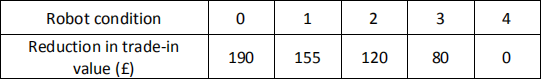
Table 2: Reduction in trade-in value for different robot conditions

The company wishes to maximise its profit over a period of 12 working days. At the end of these 12 days, the warehouse will be closed down and all robots will be sold to a third party. Use stochastic dynamic programming to find an optimal policy for carrying out robot repairs which minimises the expected sum of costs over 12 days, taking into account the repair costs, loss of productivity costs and the reduction in trade-in value at the end of the 12-day period. You should represent your optimal policy in the form of a 12 × 5 table which shows, for each day and each possible robot condition, whether or not repairs should be carried out. [15 marks]

(e) You are now told that at the beginning of the 12-day period, the conditions of the 80 robots in the warehouse are as follows: 28 robots are in state 4, 19 are in state 3, 16 are in state 2, 14 are in state 1 and 3 are in state 0.

The company has the option to use a different contractor to carry out robot repairs. This contractor will only charge £160 per robot. However, if this contractor is used, then for each failed robot the probability of returning to state 4 next day is reduced from 1 to 0.85, because there is a 15% chance that the contractor does not have the supplies available to carry out the repair. If a robot is selected to be repaired but the repair is not carried out then it still incurs a cost of £90 due to loss of productivity and should be regarded as being in state 0 at the beginning of the next day, because it has been dismantled in preparation for repair. Also note that the alternative contractor must be used for either the entire 12-day period or not at all.

By considering the expected total costs under both options, state whether or not the alternative contractor should be used. Also, suppose the alternative contractor charges £R per robot instead of £160 per robot. Find the range of values of R for which the alternative contractor should be preferred. [10 marks]

(f) Parts (d) and (e) of this question are based on finite-stage Markov decision processes where, under each state, two actions are available: “repair” and “don’t repair”. In general, does it appear that “repair” becomes a more attractive option or a less attractive option under an optimal policy as the number of stages remaining decreases (i.e. as the end of the 12-day period approaches)? Explain why this is. You may use qualitative and/or quantitative arguments in your answer. [5 marks]

Question 2 (50 marks)

A local telecoms provider has a customer service line which is always staffed by two call handlers. If both call handlers are busy, incoming calls are held in a first-come-first-served queue. However, the queue size is limited to 4 callers. If 4 callers are already waiting in the queue, then any further incoming calls are rejected and callers are asked to try again later. This means that the maximum number of callers that can be waiting on the line at any given time (including those in service) is 6.

Furthermore, customers are impatient and may ‘hang up’ if they are forced to wait in the queue for too long. You may assume that customer i (for i = 1, 2, 3, … ) is only prepared to wait in the queue for a maximum of Ti minutes before hanging up, where Ti is an exponentially-distributed random variable with a rate parameter of . This means that every customer has their own randomly-distributed ‘patience limit’, but the patience limits all have the same distribution. Another way of expressing this is that each customer in the queue is abandoning the system at a rate of per minute. Note that customers do not abandon the system if they have already entered service.

You may also assume that, during normal working hours, incoming calls arrive according to a Poisson process with a rate of per minute, and all service times are independently and exponentially distributed with a rate of per minute.

(a) Use the information above to formulate the process of calls entering and leaving the customer service line as a continuous-time Markov chain (CTMC). You should specify the state space of the CTMC and also provide the full generator matrix in terms of the parameters , and .

Is this CTMC a birth-death process? Explain your answer. [10 marks]

(b) The spreadsheet Q2_data.xslx shows the evolution of the process between 10AM and 4PM on a particular day. The information provided includes the times at which calls arrived, the lengths of the service times and the times at which callers abandoned the system (where applicable). Note that all times have been rounded to the nearest hundredth of a minute. Also, service times can sometimes be very short; this can happen if calls are forwarded to another department (e.g. technical support).

Use this dataset to estimate appropriate values of , and for the CTMC formulated in part (a). Also comment on whether or not the assumption of exponential service times appears to be correct. [10 marks]

(Hint: to estimate , you may find it useful to look up methods for estimating exponential rate parameters when you have censored data.)

(c) Let denote the steady-state probability of the CTMC being in state i. Use your values of , and from part (b) to calculate for i = 0, 1, 2, 3, 4, 5, 6. [5 marks]

(d) Use your estimated value of and the steady-state probabilities in part (c) to calculate the expected number of ‘abandonments’ in a typical hour, i.e. the expected number of customers who hang up due to impatience. [5 marks]

(e) Suppose that, at 12:00PM, there are 2 customers on the line; i.e. both call handlers are busy and no calls are waiting in the queue. Calculate the probability that

(i) no state transitions (either arrivals or service completions) happen within the next two minutes;

(ii) at least one service is completed before the next customer arrival;

(iii) both services are completed before the next customer arrival.

[10 marks]

(f) Six months later, the company has retrained its customer service staff so that they now follow a more detailed “script” when dealing with callers’ requests. The company believes that, with this new method of handling calls, service times (in minutes) follow an Erlang distribution with probability density function

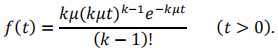
You may also assume that the shape parameter is k = 2 and the scale parameter is the same value of that you estimated in part (b).

Under the new service time distribution, do you think it is still possible to formulate the system as a CTMC? If your answer is “yes”, you should carefully explain how the system state should be defined in the new CTMC (but there is no need to provide the generator matrix). If your answer is “no”, you should explain why this is not possible. [5 marks]

(g) In the new version of the system described in part (f), do you think the proportion of customers who abandon the system due to impatience will be higher or lower than it was in the original system? Explain your reasoning. [5 marks]

Question 3 (50 marks)

At a large post office in a city centre, customers collect tickets upon arrival and wait until their ticket number is called by one of the clerks at the service counters. This process can be modelled as a first-come-first-served queue with multiple servers. It is believed that arrivals can be modelled as a nonhomogeneous Poisson process, and all service times are independently and exponentially distributed with a rate = 0.4 per minute. Tables 3 and 4 show how the arrival rate per minute and the number of clerks on duty vary between 8AM and 2PM on a typical working day.

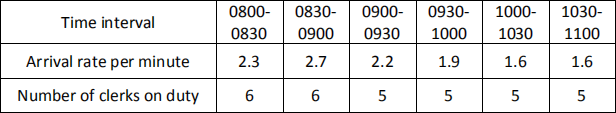
Table 3: Arrival rates per minute and numbers of clerks on duty between 8AM and 11AM

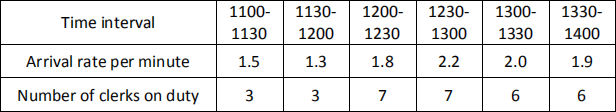
Table 4: Arrival rates per minute and numbers of clerks on duty between 11AM and 2PM

(a) Use a normal approximation to estimate the probability that more than 250 customers arrive between 8AM and 10AM. [5 marks]

(b) Use the pointwise stationary approximation (PSA) to estimate the expected waiting time in the system for a customer who arrives at 10:15AM. Also, suppose we use the PSA again to estimate the expected waiting time in the system for a customer who arrives at 10:45AM. Which of these two estimates (10:15AM or 10:45AM) do you think is likely to be more accurate? Explain your reasoning. [5 marks]

(c) Use the method of numerical integration to estimate

(i) the expected number of customers in the system at 11:50AM;

(ii) the probability that more than 10 customers are in the system at 11:50AM;

(iii) the expected waiting time in the system of a customer who enters the system at 11:50AM.

You may assume that there are no customers in the system at 8AM.

How reliable do you think your expected waiting time estimate in part (iii) is? Do you think it is more likely to be an overestimate or an underestimate of the true value? Explain your reasoning. [10 marks]

(d) The post office management team are considering making changes to the numbers of clerks on duty in the hours between 8AM and 2PM. They have 32 clerk hours available during this period, which are currently being allocated as shown in Tables 3 and 4. For each hour (0800-0900, 0900-1000, etc. up to 1300-1400) they can choose how many clerks should be on duty, but the total number of clerk hours must be 32. They would like to minimise the average number of customers in the system during the entire period from 8AM to 2PM.

By using numerical integration to estimate the average number of customers in the system under different possible allocations for the numbers of clerks on duty per hour, find the best allocation that you can. You should fully explain your method(s) and the different allocations that you have tried, and also report the results for each allocation. Note that the number of clerks on duty can be changed at the start of each hour, but not within a particular hour. [12 marks]

(e) Now suppose the post office has been redesigned so that customers who require the foreign exchange service are directed to a separate single-server queue instead of collecting a ticket. You may assume that 10% of customers arriving at the post office require the foreign exchange service, and (hence) arrivals to the single-server queue can be modelled as a nonhomogeneous Poisson process with arrival rates equal to one tenth of those shown in Tables 3 and 4 (i.e. 0.23 per minute between 8AM and 8:30AM, 0.27 per minute between 8:30AM and 9AM, etc.).

Service times (in minutes) at the foreign exchange service have a triangular distribution with a minimum value a = 0.5, maximum b = 8 and mode c = 2.

Use a simple stationary approximation (SSA) to estimate the expected number of customers in the queue for the foreign exchange service (not including customers being served) and also the expected waiting time in the queue between 8AM and 2PM. [8 marks]

(f) This part requires you to undertake some further reading.

An alternative method for estimating performance measures in time-dependent queues is called “discrete time modelling” (DTM), originally developed by researchers at Lancaster University during the 1990s. This method is described in the following research papers:

• D.J. Worthington and A.D. Wall. 1999. Using the discrete time modelling approach to evaluate the time-dependent behaviour of queueing systems. Journal of the Operational Research Society 50 : 777-788.

• A.D. Wall and D.J. Worthington. 2007. Time-dependent analysis of virtual waiting time behaviour in discrete time queues. European Journal of Operational Research 178 : 482-499.

(i) Explain briefly (in 100 words or less) how the discrete time modelling method works. You must provide an explanation using your own words. Do not copy any phrases or sentences from the articles above, or anywhere else.

(ii) Briefly describe (in 100 words or less) some of the main advantages of the discrete time modelling approach. You may find it useful to think of comparisons between DTM and other methods that have been considered in this module for analysing time-dependent queues such as the SSA, PSA and numerical integration.

[10 marks]