Assignment: Homework 3

Due: March 4th

#1: For this problem, you should remind yourself of the definition of the Hardy-Weinberg equilibrium. Assume the base assumptions for our population, i.e., it

(A0) is diploid (2 alleles A and a),

(A1) has random mating,

(A2) has non-overlapping generations,

(A3) has an infinite population,

(A4) is monoecious

(A5) and has no selection, no mutation, and no migration.

Here, we found that the frequencies immediately fixate based on the initial frequencies; in particular, the process fixates at the Hardy-Weinberg equilibrium. Prove that the genotype frequencies  and are in Hardy-Weinberg equilibrium if and only if

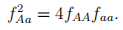
Hint 1: For proving the converse statement, i.e., showing that  implies the frequencies are in Hardy-Weinberg equilibrium, first assume that and then prove that . 

Hint 2: if and only if .

#2: (Exercise 3.2.8 from textbook) Consider a single locus with two alleles A and a. Assume our population is dioecious, i.e., each offspring has a female and male parent. Note this means the population has two sub-populations and separate frequencies for each sex. In particular, assume the frequencies  are given and assume the following of our population:

(A0) is diploid (2 alleles A and a),

(A1) has random mating,

(A2) has non-overlapping generations,

(A3) has an infinite population,

(A4) is dioecious

(A5) and has no selection, no mutation, and no migration.

(a) Calculate the genotype and allele frequencies of the first genera-tion in terms of the generation 0 genotype frequencies.

(b) Show that the allele frequencies of the male and female popula-tions are equal and constant for all generations t ≥ 1. Show that the genotype frequencies are in Hardy-Weinberg equilibrium with

in generations t ≥ 2.

#3: In the most recent pre-recordings, we went over cob-webbing (see 2/23 and 2/25 lectures). Assume that is a sequence of frequencies generated by the following difference equation:

In the four plots featured in Figure 1,

(a) find and label the fixed points or equilibria,

(b) determine their stabilities through cob-webbing (in the region shown).

In particular, for part (b), make sure to show at least two trajectories, i.e. with different initial conditions f(0), per plot; if dynamics change based on where you start your process, make sure to show it in the figure. Also, if these figures are too small for your cobwebbing (e.g., if you print this out or draw on the PDF but feel too cramped), feel free to just qualitatively hand-copy the figures to another sheet of paper.

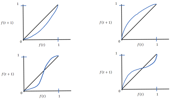
Figure 1: Purple curve is (f) and the black line is the line on which f(t+1) = f(t).