ENSC 180: Introduction to Engineering

Analysis

School of Engineering Science, Spring 2020

Copyright © 2020 W. Craig Scratchley – all rights reserved

Assignment #1

Due 8 February 2020, 2:20 pm.

Please do not make any change to the names of files and functions provided to you when you submit your code. 

Question 1:

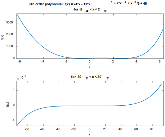
Plot the following mathematical functions using the "fplot" and “subplot” functions of MATLAB for MATLAB domains  (on the top of the figure) and  (on the bottom of the figure). The title of the top plot should include the mathematical function and type of function on the top line and the MATLAB domain (as a string) on a second line (as shown in the example, below). The title of the bottom plot should just include the MATLAB domain. Please ensure the x and y axes are properly labelled exactly as shown in the example. The drawing of the plots for a mathematical function should be done in the plot2domains function, in the plot2domains.m file. The function should return an array of 2 function line objects, one for each call to fplot. Call the plot2domains function for each mathematical function provided in MATLAB symbolic form, and think about what you see. The expected output figure is given for Question 1a. (15/100)

a) 5th order polynomial:

b) trigonometric function:

c) exponential function:

d) logarithmic function:

Question 2:

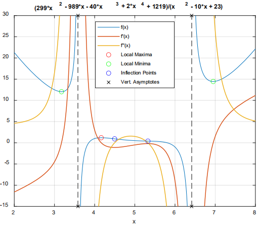
Using the "fplot" function of MATLAB, plot the following mathematical function, its first and second derivatives in one figure and in that order. x limits for the plot should be 2 to 8, and vertical (y) limits for the plot should be -15 to 30. Identify all local maxima, local minima, inflection points, and vertical asymptotes of the mathematical function. After plotting the three lines, circle all the local maxima in red, all local minima in green, and all the inflection points in blue. Vertical asymptotes should be indicated with black ‘x’s on the bottom and top borders as shown (the fplot function of MATLAB draws dashed lines for the vertical asymptotes automatically). Each type of point must be drawn in the order identified above. For each type, all points of that type must be plotted all at once except for the ‘x’s for the vertical asymptotes, for which the bottom ‘x’s should be plotted before the top ‘x’s. Please include the title, x axis label and legend in the plot that are identical to those shown in the Figure below. The implementation of these requirements should be done in a function in a file Q2.m. Function Q2 takes no input and returns the following:

Output = {fplotH; lmaxPlot; lminPlot; inflPlot; verAsymPlotBottom};

where fplotH returns the function line object returned for the plot of f(x), and the other objects are the lineseries/line objects returned for the plots of the local maxima, local minima, inflection points, and the bottom markers for vertical asymptotes. (40/100)

rational function:

Question 3:

Create a MATLAB function that plots with fplot a mathematical function with limits for x determined according to the instructions below. The function should be implemented in the auto_fplot.m file provided.

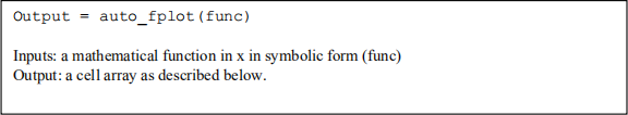
This auto_fplot function should meet the following requirements.

1) After the mathematical function has been plotted, the auto_fplot function should be able to plot a set of interesting points (i.e. local maxima, local minima, inflection points, and two points for each vertical asymptote) for as many types of functions as possible. These should work for any polynomial equation. Vertical asymptotes should work for any rational function. All local maxima should be indicated with red circles, all local minima should be indicated with green circles and all inflection points should be indicated with blue circles. Vertical asymptotes should be indicated with black ‘x’s on the bottom and top borders (the fplot function of MATLAB draws dashed lines for the vertical asymptotes automatically). Each type of point must be drawn in that order if that type of point exists for the mathematical function. For each type, all points of that type must be plotted all at once and only if at least one point of that type exists. The “region of interest” or “domain of interest” (i.e. portion between the two extreme “interesting” points if there is a finite number of such points) should be in the middle and occupy 70% of the x limits of the plot. If there is no “interesting” point found (or an infinite number of interesting points1), plot the mathematical function and set the limits of x to be from . And if there is only one interesting point, xinteresting, then set the limits of x to be

from .

Function auto_fplot returns the following:

Output = {fplotH; lmaxPlot; lminPlot; inflPlot; verAsymPlotBottom};

where fplotH returns the function line object returned for the plot of f(x), and the other objects are the lineseries/line objects returned for the plots of the local maxima, local minima, inflection points, and the bottom markers for vertical asymptotes.

2) The mathematical function as a title, axes labels (i.e., ‘x’ for x axis and ‘f(x)’ for y axis) and legend (i.e., ‘f(x)’, ‘Local Maxima’, ‘Local Minima’, 'Inflection Points', and ‘Vert. Asymptotes’ as needed) should be included in the plot. Please make sure all your strings match these instructions. Only include in the legend those types of interesting points that exist for the mathematical function being plotted. These legend entries should be shown as plural even if there is only one point of a certain type.

3) Please complete the help comments at the top of the file. Do not modify the characters

“%output = AUTO_FPLOT (f” before the “…”

Bonus requirements:

4) Can you include the location of any horizontal asymptotes? A left horizontal asymptote can be plotted as a green ‘x’ on the left border, and a right horizontal asymptote can be plotted as a red ‘x’ on the right border. Plot the left horizontal asymptote value, if it exists, after all points mentioned in paragraph 1 above, and plot the right horizontal asymptote value, if it exists, last. Depending on which horizontal asymptote(s) may or may not exist, the legend can have entries “Left Asymptote” and/or “Right Asymptote” (note that these are grammatically singular).

5) (a) If the input is a periodic function, plot 2 periods of the function including the point f(0) (b) try to plot maxima, minima, inflection points, and vertical asymptotes in the 2 periods as described in paragraph 1 and (c) hopefully with a periodic maximum at the left and right borders of the plot.

6) If you believe that some “interesting” points exist, but you cannot solve for them symbolically, just remove those interesting points from the collection that you are considering and then apply the rules to any remaining interesting points to determine the x limits of the figure.

Your implementation will likely be evaluated using a set of test functions, and some mathematical test functions may be provided. In any case, write your own mathematical functions to test your auto_fplot function against. Your auto_fplot function should work for any reasonable mathematical function, especially simple functions. You have been warned! For now, you can test your auto_fplot function with mathematical functions including those shown in Question 1 and Question 2. Students in the class are highly encouraged to share their mathematical testing functions on Piazza. You can also include your output figures for other students to compare with.

(45/100 + 15 bonus)