Physics 411: Homework IV

Due Tuesday Feb 23, 2021

Emanuel Gull

Romberg Integration

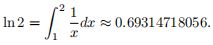
Romberg integration often gives very precise results for comparatively few function evaluations. In this exercise you will implement the integration method and illustrate its precision. As an example we use the function

1. Implement a function that computes a sequence of trapezoidal integrals with step size for i up to m, , as described in the lecture. Make sure you reuse data from i - 1 for obtaining the ith integral. Your function should return the estimates , . . . , .

2. Implement a function that computes all Romberg coefficients with p ≤ m, q ≤ p, given the output of task 1.

3. Make a table in which entry (p, q) corresponds to the Romberg estimate for the integral mentioned above. use m = 5. Show in a plot how the relative error of the integration converges as a function of h (use the best Romberg estimate and plot it on a log-log scale).

For full credit hand in the program, the table of coefficients, and a plot of the relative errors. Make sure your curves and axes are properly labeled and the data is clearly visible.

Spline Interpolation

1. On CTOOLS you will find raw data for the monthly temperature values at the University of Michigan since 1891 in the file ‘climate.txt’. Write a program that reads in the data as provided in the file and selects the last five years of extreme minimum daily temperature available. The data format is

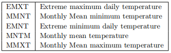
and contains additional header data. Plot the data points as points and label your axes and curves.

2. Using the Python handout and the help pages of scipy.interpolate.splrep and scipy.interpolate.splprep prepare a spline interpolation through the temperature curve. Plot it using a fine grid and a continuous line.

For full credit turn in printouts of your program and printouts of the plots you created. Make sure all curves and axes are properly labeled and the information contained in the data files is clearly visible.

Finding Eigenvalues

The QR matrix decomposition is implemented in numpy as numpy.linalg.qr. We will use successive QR steps to iteratively diagonalize a matrix for a quantum mechanical system.

1. The Hamiltonian of the harmonic oscillator is

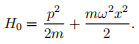
In dimensionless units (m = 1, w = 1) its energy levels are given by

The Hamiltonian of the anharmonic oscillator is

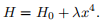
Expressed in the eigenbasis of the harmonic oscillator, and we can use this to express H in the eigenbasis of . Implement a function that generates the matrix for a matrix of size k and then computes H for a given value of λ. , the Hamiltonian of the harmonic oscillator in its eigenbasis, is given by Check that for k = 4 you obtain

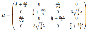
2. Implement a function that applies successive QR decompositions (use a packaged routine for the QR decom-position) to diagonalize this matrix, until the off-diagonal entries are below a given threshold (use as a threshold).

3. Plot the value of the lowest two eigenvalues as a function of λ for small λ < 0.1 and for k = 4. This will describe how the system reacts to a small anharmonic perturbation of perturbation strength λ. As you make k larger, your result will get more and more precise. Make a plot that shows how your results change as you increase k.

For full credit turn in printouts of the programs and your plots.

LU decomposition

1. Write a function that takes a matrix A and returns two matrices L and U such that A = LU, with L a lower left triangular matrix with 1 on the diagonal and U an upper right triangular matrix. You do not need to implement pivoting.

2. Test your function for the matrix

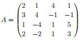
For full credit hand in a program that performs the LU decomposition, a printout that shows all intermediate steps, and the final matrices L and U.