Project 01: The Wave Equation

Version: Current as of 2021-02-04 10:08:52

Due:

– Preparation: 2021-02-02 23:59:00

– Coding & Analysis: 2021-02-12 23:59:00 (24 hour grace period applies to this due date.)

Points: 100

Deliverables:

– Preparation work as a PDF, typeset with LaTeX, through Canvas.

– All code through code.vt.edu, including all LaTeX source.

– Project report and analysis as a PDF, typeset with LaTeX, through Canvas.

Collaboration:

– This assignment is to be completed by yourself.

– For conceptual aspects of this assignment, you may seek assistance from your classmates. In your submission you must indicate from whom you received assistance.

– You may not assist or seek assistance from your classmates on matters of programming, code design, or derivations.

– If you are unsure, ask course staff.

Honor Code: By submitting this assignment, you acknowledge that you have adhered to the Virginia Tech Honor Code and attest to the following:

I have neither given nor received unauthorized assistance on this assignment. The work I am presenting is ultimately my own.

References

● The Wave Equation:

– General overview

✯ https://en.wikipedia.org/wiki/Wave_equation

✯ https://mathworld.wolfram.com/WaveEquation.html

✯ OpenStax: Mathematics of Waves (link)

– Standing Waves (especially in 2D with a rectangular boundary)

✯ https://en.wikipedia.org/wiki/Standing_wave

– Chapter 5.1 of Gilbert Strang’s course notes “5.1 Finite Difference Methods”

✯ https://math.mit.edu/classes/18.086/2006/am51.pdf

– Chapter 5.3 of Gilbert Strang’s course notes “5.3 The Wave Equation and Staggered Leapfrog”

✯ https://math.mit.edu/classes/18.086/2006/am53.pdf

● LaTeX:

– Writing pseudo-code in Latex: https://en.wikibooks.org/wiki/LaTeX/Algorithms

– General topics: https://www.overleaf.com/learn

● Python:

– Python 3.8 Documentation: https://docs.python.org/3/

– NumPy Documentation: https://docs.scipy.org/doc/numpy-1.17.0/reference/

– SciPy Documentation: https://docs.scipy.org/doc/scipy-1.4.1/reference/

– MatPlotlib Documentation: https://matplotlib.org/contents.html

Background

This semester, we will explore the wave equation, a partial differential equation (PDE) that describes the temporal evolution of a wave in a physical medium. We will write a numerical code for simulating solutions to this equation. You will not need any prior knowledge of the wave equation, PDEs in general, or numerical solvers for PDEs to complete these projects.

      In this first project, we will develop some understanding of the wave equation and how finite difference approximations induce a time-stepping algorithm (recurrence) for numerically solving this equation. We will make our first pass at implementing the algorithm in Python. Our first implementation is in a language designed for rapid prototyping because we are more concerned with getting the algorithm correct than we are about performance.

      We will work with the 2-dimensional, isotropic acoustic wave equation,

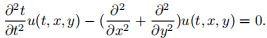
If this looks complicated, don’t worry, we will simplify the notation shortly. This equation describes the propagation of acoustic pressure waves u(t, x, y) through an acoustic medium (e.g., air or water). (We’ve implicitly set the speed of sound to 1, but you can ignore that for now.) We see here that the solution, the pressure field, is a function of both space and time and that the second time derivative of the solution is equal to the sum of the two second spatial derivatives.

      In the remaining parts of this assignment (and in discussion in class) we will use a more compact notation. Eq. 1 can instead be written,

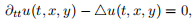
where ∂tt a shorthand for the second partial derivative in time and 4 = ∂xx + ∂yy is called the Laplacian, the sum of the second partial derivatives in space.

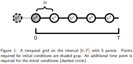
      The solution to this equation (u) varies with both time and space, so to solve this problem numerically (to solve on a computer) we will have to discretize it in both time and space. First, we will focus on discretizing the problem in time, so ignore the spatial dimension for now. To compute the solution over the interval [0, T], we will discretize the time dimension over nt points, spaced δt seconds apart, which we index with k, as shown in Fig. 1. Note, the notation δt references a single variable describing a small length of time and is it is not a product of δ and t.

      To further simplify notation, we use that t = kδt to define uk(x, y) = u(t, x, y). Then, the second time derivative can be approximated with a centered finite difference operation,

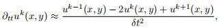
which induces the recurrence relation that we will use to solve Eq. 2,

We can compute uk+1 using knowledge of two previous solutions. To start the recurrence, we will need two initial solutions, one at t = 0 and one at t = =δt. Hence, this sort of problem is known as an initial value problem.

      The solution at each time step will be defined on a discrete spatial grid over a rectangular domain, as shown in Fig. 2. At any interior grid index, assuming δx = δy, the discrete approximation to the Laplacian is

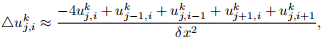
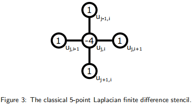
where we replace the (x, y) coordinates with grid indices such that x = iδx and y = jδy. Be careful, our indexing scheme is ordered [j, i] to following an array-like scheme, where the y-dimension maps to the columns of an array (so j selects the row) and the x-dimension maps to the rows (so i selects the column). Equation 5 manifests the classical 5-point stencil, shown in Fig 3. Try to visualize or draw how the access pattern for evaluating Eq. 5 matches this stencil.

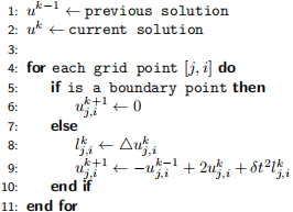
We specify the interior points separately from the boundary because this stencil would go over the edge of the grid for boundary and corner grid points. We cannot uniquely compute solution at these boundary points using the information provided so far: we have to specify the solutions at these points through boundary conditions. For this project, we will assume that the solution uk j,i = 0 if j or i are on the boundary of the grid. (This type of boundary condition is known as a homogeneous Dirichlet boundary.)

    All of this comes together to produce an algorithm for solving the wave equation. Pseudocode for the algorithm for computing a single timestep is given in Alg 1.

Algorithm 1 Algorithm for computing uk+1 .

Code Environment

● You may use the command-line interface to IPython/Jupyter or Jupyter Notebooks to implement your solution. If you use Jupyter Notebooks, you must export your solution to a Python file for submission.

● You are strongly encouraged to develop your solution using IPython from the command line.

● You do not have to do your programming on ARC for this assignment, but you still must actively use Git in your development process. You may work on your local computer or on ARC.

– To access Jupyter notebooks on TinkerCliffs:

1. Go to OnDemand (https://ood.arc.vt.edu/) and under “Interactive Apps” select “Jupyter Notebook –Container”.

2. Enter our allocation name for “account”

3. Select “normal q” or “preemptable q” for “Partition”

4. Select a sensible number of hours, 1 node, 1 core per node, and 0 GPUs

5. Click the “Launch” button

6. Open the session when it is available, close it and release the job when you are done

– To use Anaconda on ARC from the command line:

> module load Anaconda3

● For Coding Task 5, you may need ffmpeg. From the ARC command line you can access this with

> module load FFmpeg

● All necessary code must be put in your class Git repository.

● Your Git repository must have the following structure:

   

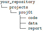
● Data and any scripts which are necessary to recreate your data, must be in the data directory.

● Your tex source for project preparation and final report go in the report directory.

● Remember: commit early, commit often, commit after minor changes, commit after major changes. Push your code to code.vt.edu frequently.

● Any code supplied by the instructor is in the course materials repository. For this project, it is also posted on Canvas.

Requirements

Preparation (20%)

The preparation for this project is to be completed in advance of the programming work. This will be handed in via Canvas as a PDF that must be generated using LaTeX. I know that LaTeX may be very new to you, but do your best here.

Tasks:

1. Assume that the problem domain is given by the rectangular domain [a, b]×[c, d], where [a, b] is the interval on the x-dimension and [c, d] is the interval on the y-dimension and that there are Nx points in the x-dimension and Ny points in the y-dimension. Derive expressions for computing δx and δy, the grid spacing in the x- and y-dimensions.

2. Give a compound logical statement (i.e., what goes in an if statement) for determining if a given grid point index [j, i] is on the boundary of the domain. Remember, we are using array indexing, so j corresponds to the y-dimension and i corresponds to the x-dimension (see Fig. 2). You may assume that there are Nx points in the x-dimension and Ny points in the y-dimension.

3. Assuming δx = δy, derive the expression for computing the discrete Laplacian at the [j, i] grid point (Alg. 1, Line 8), given in Eq. 5. Hint: You will need to apply the centered difference from Eq. 3 to each spatial dimension.

4. How might you iterate over each grid point? (Alg 1, Line 4)

5. Research an application of the wave equation. Give bullet points describing:

● How the wave equation applies to the problem you selected;

● Why you found the application interesting;

● Any differences between our formulation of the wave equation and the one in your application.

Be sure to list your sources.

(continued)

Coding (60%)

The source code for your solution is to be submitted via GitLab. Include a README file in your source directory with instructions for how to run your code.

Assumptions:

● Assume that all solutions uk for an n × n grid are described by an n × n NumPy array.

● The problem domain will be the unit square [0, 1] × [0, 1].

● You are strongly encouraged to write other functions or break the assigned functions into smaller parts.

Tasks:

1. Implement a function that evaluates the standing wave solution to the wave equation (see References for more details),

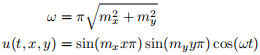
on the computational grid. The variable t is the current time in the simulation and the variables mx and my control the number of nodes in the standing wave (unrelated to the number of grid points). These variables should be arguments to your function, which will let you generate your initial conditions.

2. Implement a function that computes one time step of the wave equation simulation.

3. Implement a function that, given the final simulation time T, the grid size n, and the number of stationary nodes mx and my, computes and returns nt iterations of the simulation.

● For numerical reasons, use δt = αδx/√2, for α = 1. (We will vary α in the analysis.)

4. You are provided with functions that use Matplotlib to make 2D and 3D animations of the evolution of the wavefields. Modify these routines to ensure that they are correctly oriented, have axis labels, have correct axis ranges, and show the simulation time on each frame (not the running time!).

Analysis (20%)

Your report for this project will be submitted via Canvas. Tex source, images, videos, and final PDFs should be included in your Git repositories.

Tasks:

1. Select an interesting mx > 1 and my > 1 such that mx = my. Time your code for computing solutions for T = 5 and n = 11, 26, 51, 101, 201, and 301. The last one may take a while. Be sure to time the total simulation time only (including initialization). Record δx, δt, and nt for each setup. Make a table with the total run-time and the average time per time step. Plot both timings as a function of N = n × n.

2. If n = 100, 000 and T = 5, how many time steps are required for a stable solution? What percentage of the total simulation will 100 iterations solve? Based on your results from the previous question, estimate how long it will take to run just 100 iterations for n = 100, 000. You should not need further experiments but may need to devise and fit a model to answer this question. Justify your estimate and choice of model.

3. For T = 5 and n = 11, 101, and 201, include images of the solution near t = 1, t = 3, and t = 5.

4. Let T = 5, n = 101, mx = 2, my = 3. Run simulations for α = 1.0 and α = 1.001.

(a) You should see the latter solution “blow up” due to numerical instability. At what time do you start to see this behavior?

(b) Create videos of the evolution of the system in both cases. You may use the Matplotlib FuncAnimation routine’s movie writer (which requires the ffmpeg tool) or a screen recorder (e.g., Zoom or Kaltura Capture) to record the video. Upload the video to Canvas.