EC 508, Econometrics

Jean-Jacques Forneron

Boston University

Problem Set 2: Testing Hypotheses with OLS

due Monday February 22, 2021

Instructions: Submissions are individual, R code must be readable, commented and attached at the end of your problem set. Plots, tables and other outputs should be given in the answers or at the end of the problem set.

Problem 1: Suits

The data set in lawsch85.dta contains information for 1985 cohort of the top 156 law schools in the US. Variables in the dataset include rank, law school ranking, salary, median starting salary, cost, law school cost.

i. Compute the average starting salary across law schools in the sample. Do you think it coincides with the average starting salary across law students?¹

ii. Regress starting salaries on the law school’s ranking:

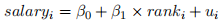
compute standard errors and a 95% confidence interval for . Report your results.

iii. What is the expected difference in starting salary between the 20th top law school with the 40th top law school? Construct a 95% confidence interval for the difference. Report your results.²

iv. Now regress the cost of attending law school on the school’s ranking:

compute standard errors and a 95% confidence interval for . Report your results.

v. What is the expected difference in cost between the 20th top law school with the 40th top law school? Construct a 95% confidence interval for the difference. Report your results.

¹Hint: think about the size of different schools and the law of iterated expectations

²Hint: the standard error for 2 is 2se(). More generally, for any number ∆, the standard error for ∆ is |∆|se(); standard errors cannot be negative.

vi. Given the results in ii-iii. and iv-v. discuss the relative benefits and costs of attending a more prestigious program.

vii. Construct a plot with rank on the x-axis and cost on the y-axis. Do you believe Least-Squares Assumptions (LSA) 1-3 are reasonable assumptions in this setting? Plot rank against salary in the same manner and comment on LSA 1-3.

viii. Construct a plot with rank on the x-axis and log(salary) on the y-axis.³ Comment on LSA 1-3.

ix. Repeat ii. but this time regressing log(salary) on rank:

compute standard errors and a 95% confifidence interval for .

Remark: This is still a linear model as we saw in class, everything we have seen so far applies to this regression. The only difference is in the interpretation of , when x is a continuous regressor:

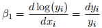
because d log(x) = dx/x. This means that 100× is (roughly) the percentage increase in y when x changes by one unit. Economists often look at log(salary) instead of salary to make statements in terms of percentage increases/decreases. Here x is discrete, so 100 × is just the percent change in log(salary) when we change rank by one unit.

Problem 2: Real Estate

The data set hprice1.dta contains observations on the selling price, in thousands of dollars, and features of houses sold in a given area, including bdrms, the number of bedrooms and, sqrft, the size of house in square feet. For more details on the variables in the dataset, see hprice1.des.

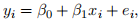
i. Estimate the following regression model:

and report the estimated coefficients, standard errors.

ii. What is the estimated increase in price for a house with one more bedroom, holding square footage constant? Compare this number to the average selling price and discuss the magni-tude of this increase.

iii. Using a 95% confidence interval, determine whether this increase statistically significant? Explain why this result is, or is not, intuitive.

³log(salary) is already present in the dataset as lsalary but you could also construct it using data$lsalary = log(data$salary).

iv. What is the estimated increase in price for a house with an additional bedroom that is 140 square feet in size? Compare this to your answer in part (ii).

v. Is the effect of the size of house alone statistically significant? Explain why this result is, or is not, intuitive.

vi. The first house in the sample has 2,438 square feet and 4 bedrooms. Find the predicted selling price for this house from the OLS regression line.

vii. The actual selling price of the first house in the sample was $300,000 (so price is 300 in the data). Find the residual for this house. Does it suggest that the buyer underpaid or overpaid for the house?

Problem 3: Omitted Variables

Consider the true population model:

(1)

where has mean zero and is independent of both and . Some notation: var() = , var() = and cov(, ) = . (, , ) are iid and have finite fourth moments. Assume and have mean zero.

i. Suppose an economist regresses on only, omitting zi . Should she/he be concerned about the validity of the Least-Squares Assumptions? Explain.

ii. He/she decides to proceed regardless of your previous answer and estimates the following model:

(2)

with as an error term in the regression formula. Note that = + . Write down the OLS formula for with only as a regressor. Substitute in this formula using (??). Express as the sum of and an another term.

iii. Express the probability limit of - β1 using the law of large numbers. The limit depends on the following terms: , and . This is the so-called omitted variable bias.

iv. Suppose the economist finds a positive effect: > 0. You know that > 0 and < 0. What can you tell him/her about the true using this information?

v. You will now conduct a numerical experiment to see the effect of omitted variable bias on the coefficients. To fix the random numbers, so that everyone gets identical results, type set.seed(123) at the beginning of your R code.⁴ Then, using rnorm and setting n = 1, 000,

⁴Every time you run set.seed(123) in R, it re-sets the random numbers to the same sequence. There is nothing special about 123, set.seed(666) would set another deterministic sequence.

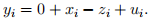
draw ∼ (0, 1) , ∼ (0, 1) and compute = + , ∼ (0, 1) for i = 1, . . . , n. This implies that: = 1, = 1. Now generate:

With the lm function, compute the OLS estimates when regressing only on . Use coeftest to test for H0 : = 0 using the single regressor specification.⁵

vi. Explain your result above in light of your earlier findings. To do this, you should compute the omitted variable bias using the formula you derived by hand in iii.

⁵Do not forget to use vcovHC.