STA238 - Winter 2021

Assignment 2 Instructions

Samantha-Jo Caetano

Instructions

This is an individual assignment. You are expected to work on this independently. You are more than welcome to discuss ideas, code, concepts, etc. regarding this assignment with your class mates. Please do not share your code or your written text with your peers. It is expected that all code and written work should be written by yourself (unless they are taken from the materials provided in this course or are from a credible source which you have cited). Please note, this assignment is fairly open, so the context of most of the work completed here should not match your peers.

There is a starter Rmd file (called Assignment2.Rmd) available for you to use to start your code. There is also some example code for Part 1 Step 2 in the Assignment2-Part1-Step2-Example.Rmd file.

Submission Due: Friday February 12th at 11:59pm ET

Your complete .Rmd file that you create for this assignment AND the resulting pdf (i.e., the one you ‘Knit to PDF’ from your .Rmd file) must be uploaded into a Quercus assignment (link: https://q.utoronto.ca/courses/204754/assignments/551279) by 11:59PM ET, on Friday, February 12th. Late assignments are not accepted. Please consult the course syllabus for other inquiries.

Assignment grading

There are two parts to this assignment. One is theory-based and the other is data analysis and communica-tion/writing focused. We recommend you spellcheck and proofread your written work. We will be directly marking the pdf files, thus please ensure that your final submission looks as you want it to look before submitting it.

As mentioned above, this assignment will be marked based on the output in the pdf submission. You must submit both the Rmd and pdf files for this assignment to receive full marks in terms of reproducible.

This assignment will be graded based off the rubric available on the Assignment Quercus page (link: https://q.utoronto.ca/courses/204754/assignments/541878). TAs will look over each section and select the appropriate grade for that section based off a coarse overview (one-time read over) of that section. Your assignment should be well understood to the average university level student after reading it once. I would suggest you make sure your document looks clean, asthetically pleasing, and has been proofread. You will be able to see the rubric grade for each section. There may be some comments/feedback provided (by the TAs) if the same issue seems to be arising in multiple sections, but you will likely receive no comments/feedback (due to the scaling of the class and marking).

Part 1

Description

Recall from Chapter 16 that the sample variance is defined as: 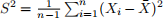 and usually one of the common questions regarding this variance formula is “Why are we dividing by n - 1 and not n?”. We will investigate this here.

Step 1 (Mathematical Justification):

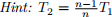
Let’s compare the following two estimators:

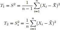
Find the expected value of each of these estimators and state whether they are unbiased or biased in estimating the population variance . 

Step 2 (Simulation Justification):

Compare the bias, variance and mean squared error (MSE) of the two estimators based on simulated samples (see the materials covered in the Weeks 3 & 4 synchronous lecture as well as Ch. 4 & 5 of the Supplementary Materials). Make sure to comment on which is the ‘preferred’ estimator (or if it’s not clear be sure to discuss the tradeoffs between the two estimators). Please use the last 3 digits of your student number to set the seed for your simulation.

It is recommended that for the simulation you assume that . If you wish your data to follow a different distribution that is fine, but be sure to state which distribution you are simulating from. You can use a sample size of n = 100 and a number of simulations to be M = 1000.

Be sure to demonstrate this graphically. Create a set of 3 plots (or 3 tables) to make your comparisons (1 for bias, 1 for variance, 1 for MSE for each estimator). Each plot should mimic Figure 20.2 or 20.3 (p. 306) of MIPS (again for each of the bias, variance and MSE for each estimator). Make sure to comment on each table/plot and describe what it is demonstrating in terms of comparing between  and .

General Notes (for Part 1):

•  This question is open book, so you can use outside sources (i.e., textbooks, academic papers, credible websites, etc.), especially in Step 1, to prove/show the biased/unbiasedness properties. Just make sure you properly credit any outside sources.

•  If you intend to mimic Figure 20.3 I would recommend running the simulations for a handful of different values of the population variance (e.g. = 1, 2, 3, 4, 5). This is optional.

•  You will likely need to use LaTeX code in your Rmd file. Please have a look at our course Resources page, as well as the synchronous lecture in Week 4.

•  Grammar is not the main focus of the assessment, but it is important that you communicate in a clear and professional manner. I.e., no slang or emojis should appear.

•  You may want to include a bibliography in this section. If it is clear that you (or the reader) looked up something that is not common knowledge then you will lose points.

Part 2

Description:

In this question you will create a “Model” (or “Methods”) section and a “Results” section of a report. This will allow you to look at the relationship between two variables, and summarize a meaningful aspect of the data. Please find some data through either:

1. The Toronto Open Data Portal (https://open.toronto.ca/) and download it via the opendatatoronto R package (https://sharlagelfand.github.io/opendatatoronto/).

2. Some survey data from the 2019 Canadian Election Study (http://www.ces-eec.ca/) and download it via the cesR R package (https://hodgettsp.github.io/cesR/).

Feel free to use the same data as you did on Assignment 1, just make sure that the data is appropriate for your model.

The goal of the Model section is to introduce the reader to the model (or statistical methods) that you will be using to analyze the data.

Your Model section should include the following:

•  The mathematical model (we have only covered (simple) linear regression so far).

•  An explanation of the model for a general science reader (i.e., not a statistician).

•  A description of why the model is appropriate (based off assumptions, variable types and practical rationale).

•  In line referencing

•  In line R code (if needed).

Your Results section should include the following:

•  A well formatted and labelled table containing the numerical output of the model (i.e., the estimates from the linear regression model).

•  An explanation/interpretation of the results.

•  Some commentary on whether or not the results seem reasonable (based off the original scatterplot).

•  A scatterplot (same one as in the model section) but with the line (or curve) laid on top of it.

•  Text explaining/highlighting each table or figure.

•  In line referencing

•  In line R code (if needed).

•  Reference any packages and any software used to complete this section.

General Notes (for Part 2):

•  It is expected that your model be a simple linear regression model.

•  If you would like to you can instead opt to add in a quadratic term, or additional independent variables.

   This is not required, but may be of interest to some of you and wanted to put this out there since we did discuss it in class.

•  All tables/figures should be well labelled and clean.

•  Everything in Part 2 should be written in full sentences/paragraphs.

•  There should be no evidence that Part 2 is an assignment, I should be able to take a screenshot of this section and paste it into a newspaper/blog.

•  There should be no raw code. Any output should be nicely formatted.

•  You will also need a reference section. You should reference the data, any outside code/documentation and any ideas/concepts that are taken outside of the course.

•  Note, we are not marking grammar, but we are looking for clarity. If you need help with writing there are resources posted on the Course Info>Resources page of Quercus. It is important that you communicate in a clear and professional manner. I.e., no slang or emojis should appear.

•  Use full sentences.

•  Be specific. Remember, you are selecting this data and the reader/marker may not be familiar with it. A good principle is to assume that your audience is not aware of the subject matter.

•  Remember to end with a conclusion. This means reiterating the key points from your writing.