Lab 3B: Numerical Integration
this lab you will explore the convergence properties of the trapezoid rule. In the second part you
will explore an application of numerical integration.
Trapezoid Rule
As you have seen in Lab 3A and the midterm, the trapezoid rule for integrating a function f(x)
with n sub-intervals between a and b of width h = (b − a)/n is defined as
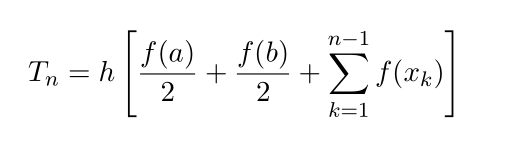
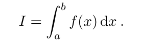
where x k = a + kh. Let the exact value of the integral be denoted
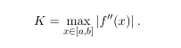
We know the error in the trapezoid rule is given by
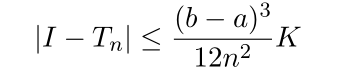
where
Part 1: Exponentially Convergent Trapezoidal Rule
For many integrals, the error formula in equation (3) provides a close bound for the actual error.
Some periodic integrals converge much faster than the error formula for the trapezoid rule. In this
problem you will be exploring a few such integrals. See [1] for an overview of the theory as well as
several examples. See [2] for a more advanced discussion.
Problem 1
Consider the integral from your midterm
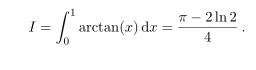
Show that the convergence rate of the forward error for this integral using the trapezoid rule is the
same as the convergence rate of the error formula (equation (3)) for the trapezoid rule. In your
report you should discuss how you know they have the same convergence rate. Use tables, plots, 3D
printed figures, holograms, etc. to convince the marker that you understand why the convergence
rates are equal.
Problem 2
Consider the integral
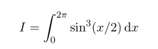
Show that the convergence rate of this integral is O(n −4 ) and not O(n −2 ) as in equation (3).
Problem 3
Consider the integral
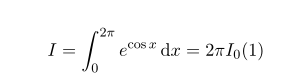
where I 0 (1) is the modified Bessel function of the first kind with ν = 0 at x = 1. This can be
evaluated in Matlab as besseli(0,1) . Show that the convergence rate of this integral is much
faster than the error formula. Again, in your report your should provide a convincing discussion
on how you know the convergence rate is faster.
Why does the forward error for this integral never do better than about 10 −15 ?
Part 2: Quadrature on Your Wrist
On a beautiful summer day your TA, Steven, was riding his Cervélo R5 road bike along the bike
paths in London 1 . Attached to the rear wheel of his bike is a sensor that can record how fast the
wheel is turning. This sensor wirelessly connects to Steven’s Garmin Forerunner 620 watch (Steven
likes running as well). Without requiring any connection to GPS or the internet, Steven’s watch
is able to accurately record the total distance biked by numerically integrating the data from the
sensor attached to the rear wheel.
In this part of the lab you will be integrating the raw data from Steven’s bike ride to estimate the
total distance he travelled. The sensor that records the rate the rear wheel is turning does not
record data points in equal time intervals. For example, if the wheel is not turning (ex. stoped at
a red light, ran into a Canadian goose on the path, etc.) the sensor will not record any points. The
Bike_Speed_Data.csv file on OWL contains the raw data. This file has two columns (you can open
it with Excel to get an idea of what is in it). The first column is the rate at which the rear wheel
is turning in revolutions per minute (RPM), and the second column is the time (in seconds) since
the beginning of the ride.
1 If you have never explored London’s bike path I highly recommend it, see
https://www.london.ca/residents/
Roads-Transportation/Transportation-Choices/Documents/2013_Bike_Map_E.pdf for a map. The yellow lines are the
paved path.
Because the trapezoid rule works with equally-spaced points, we must interpolate the raw data to
get points at equally-spaced time intervals. You will use cubic spline interpolation for this.
When using the trapezoid rule you may write your own trapezoid rule function from scratch, or
modify the trapezoid rule code given on the midterm. You may not use the trapz function in
Matlab.
You can load the data into Matlab using the csvread function.
M = csvread('Bike_Speed_Data.csv', 1 , 0 );
t = M(:, 1 ); % t is the time (in seconds) since the beginning of the ride
r = M(:, 2 ); % r is the wheels rotation in RPM
Complete the following questions and comment on the results and the procedure used in your
report.
1. Make a plot of the velocity (in m/s) vs. the time (in seconds) since the start of the ride. You
will have to convert the wheel rotation data into m/s. The diameter of the wheel is 670mm.
2. Using cubic spline interpolation, interpolate the raw data for every second along the ride.
You can use the spline function in Matlab for this. Do not use barycentric interpolation.
3. Integrate the interpolated data using the trapezoid rule to estimate the total distance Steven
biked.
4. The bike paths in London have a speed limit of 20 km/h. What is the total distance that
Steven exceeded this speed?
5. Who would win in a bike race, you or Steven? Why?
Submission Requirements
All files should be submitted on OWL on the Lab 3B submission. Submit all files needed to
reproduce the results you found in the lab.
Your report should provide a discussion of how you solved the problems and your interpretation
of the results. Your discussion should be able to convince the marker that you have a thorough
understanding of the problems and results.
References
[1] J. A. C. Weideman. Numerical integration of periodic functions: A few examples. The American
mathematical monthly, 109(1):21–36, 2002.
[2] Lloyd N Trefethen and JAC Weideman. The exponentially convergent trapezoidal rule. SIAM
Review, 56(3):385–458, 2014.
2017-03-10
In this lab you will be exploring the trapezoid rule for numerical integration. In the first part of this lab you will explore the convergence properties of the trapezoid rule. In the second part you will explore an application of numerical integration.