EC 6102 : Advanced Macroeconomic Theory Problem Set 4 Spring 2022
Hello, dear friend, you can consult us at any time if you have any questions, add WeChat: daixieit
EC 6102 : Advanced Macroeconomic Theory
Problem Set 4
Spring 2022
Instructions: Please make sure to turn in your own work. Where applicable, please print out figures and codes. This problem set is due on Tuesday, February 15.
Exercise 1
In this exercise, we will study the effects of government spending in both the RBC and New Keynesian models under a non-separable utility function as in Problem set 2:
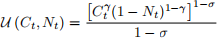
where σ > 0 and 0 < γ ≤ 1. We will work out a few details first that will help us approximate the model later on.
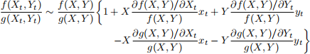
(a) Using the definition of a Taylor approximation for functions of 2 variables, show that

(b) Using the answer from question (a), show that
(c) Take the RBC model with government spending that we have studied in the lecture on the RBC model, but without private capital. Show that the optimal labor supply condition can be approximated by

where ˜σ and η˜ are functions of the Utility function with respect to private consumption/hours evaluated at steady state and the cross-derivative also evaluated at steady state. Give explicit expressions for ˜σ and η˜ as a function of parameters and/or steady state (constant) values. Remember that the time endowment for each period is normalized to 1 so that we have N ≤ 1.
(d) Now we are going to use a little trick to simplify things. Derive the resource constraint of this economy and show that under the assumption that G = 0 it can be approximated as
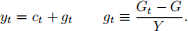
This way we can get rid of the C/Y terms in the resource constraint. Also show that the production function can be approximated as

(e) Combine all three equations and compute the solution for consumption and output as a function of the government spending shock. Given the current utility function, is it possible that the effect on consumption is positive?
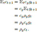
(f) We now move on to a model with sticky prices. As the model is more complex now, some expressions are going to be more involved. To make sure that this does not distract us from the main goal, we make some parameter restrictions to make things easier. In particular, we assume σ = 2. With this in mind, derive the Euler equation with respect to government bonds for this Utility function and show that it can be approximated by

Let us now make some further assumptions to simplify the model. First, since there are no endogenous state variables in this model, we know that the solution will only depend on the exogenous shocks. For example, we can write that consumption is

where cg is a function of parameters that we have to solve for. Once we have this, we can write:
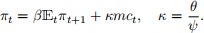
Naturally, the same goes for nt and πt. To simplify things even more, we assume that shocks have no persistence so that ρg = 0. Now that prices are sticky, we have the following Phillips curve equation
(g) Now combine both the Euler and Phillips Curve Equations and solve for the impact effect of government spending on consumption.
(h) What happens to the multiplier effect if we make prices flexible so that κ → ∞?
(i) Assuming that ˜η < 1 (which is the realistic case usually), give a necessary and sufficient condition for the multiplier effect on consumption to be positive.
Exercise 2
Now we are going to study whether the simple result that we got for the simple RBC model just now holds up when we add private capital into the picture. Take the RBC model with government spending from Lecture 2, just with the current non-separable Utility function from Exercise 1. Since we have to enter the steady state in the code, we begin with this first.
(a) Assuming again that G/Y = 0, use the labor market equilibrium condition to get a relationship between γ and N. With this expression, set γ such that we have N = 1/3 in the steady state.
(b) Simulate the effects of an increase in government spending in the full model with non-separable preferences. Tip: it is convenient to add two new variables Uc and Un that you will use in the labor supply and Euler equations. Do not forget to declare their steady state value in the parameter block and assign their value. These should feature in the initval block as well. Finally, since G/Y = 0 you will have to modify the equation for the government spending shock to be consistent with our new definition and avoid the division by 0.
(c) What about the impact on consumption now? Does our earlier conclusion hold up? Discuss
2022-02-14