MATH 3250 Written Homework 3
Hello, dear friend, you can consult us at any time if you have any questions, add WeChat: daixieit
MATH 3250
Written Homework 3
1. (Shockwave) This exercise is based on a discussion of Bernoulli equations in Advanced Engineering Mathematics by Alan Jeffrey.
Bernoulli equations can be used to model the propagation of waves in “nonlinearly elastic materials”. If a nonlinearly elastic bar receives a blow at one end (in a certain range of magnitudes), an “acceleration wave” will be created and its magnitude at time t may be modeled by a Bernoulli
equation of the following form
where µ depends on both material properties of the bar and its geometry (say, whether cross- sections are square or circular) and β depends on material properties of the bar. Because of the effects of nonlinearity, in many materials it is possible for the acceleration wave to strengthen as it
propagates to the point at which a shockwave forms, which may lead to the fracture of the bar. Let’s suppose that the magnitude of an acceleration wave in a bar is modeled by the following IVP.
The time when a shockwave forms in the bar modeled by (*) corresponds to a vertical asymptote for the graph of a = a(t), specifically, to that time t0 such that limt →t![]() a(t) = -. For the model (*), when does a shock-wave form? You’ll want to use Wolfram Alpha or Mathematica to identify this time (to several decimal places).
a(t) = -. For the model (*), when does a shock-wave form? You’ll want to use Wolfram Alpha or Mathematica to identify this time (to several decimal places).
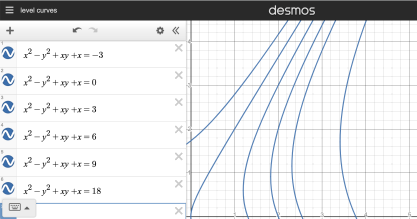
2. A metal place occupies a rectangular region in the xy-plane having vertices (0, 0), (4, 0), (4, 2), and (0, 2). The temperature T of the plate at the point (x, y) is given by

Curves along which the temperature of the plate is constant are called isotherms, and thus isotherms of the plate have equations of the form T (x, y) = c, where c is a constant. Some isotherms of our plate appear in this figure.
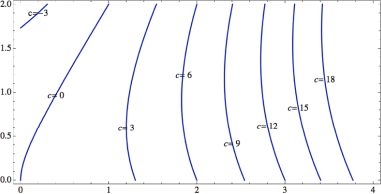
Observe that the isotherm curves x2 0 y2 + xy + x = c are implicit solutions of the equation Tx (x, y) dx + Ty (x, y) dy = 0, or equivalently,
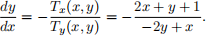
Curves orthogonal (perpendicular) to the isotherm curves are curves along which heat flows. If y = y(x) is a heat-flow curve passing through (x, y), then its slope at (x, y) must be the negative reciprocal of the quotient of (十). Thus, for a heat-flow curve, we have
Solve the preceding differential equation, finding an implicit general solution. Fixing the arbitrary constant in your implicit general solution will produce a heat-flow curve.
Extra credit. Let F (x, y) = C be the one-parameter family of implicit solutions you found for the ode (主) above. Using either Desmos or Mathematica (see instructions below), generate a graph of the isotherms (blue) and heat-flow lines (red) on the same grid. Take a screen shot of your plot and include it in your submission for extra.
● using Desmos:
At the link https://www.desmos.com/calculator/scxe341uyn, you may enter the equations as follows to produce isotherm curves like those plotted above.
Now add appropriate additional equations to produce the heat-flow lines. To change the color of curves in Desmos, long-hold the colored icon to the left of the equation. Note that your screen shot in Desmos shold be of the appropriate rectangular region with vertices (0 , 0), (4, 0), (4, 2), and (0, 2).
● using Mathematica:
Open the Mathematica Notebook “Isotherms.nb” (in the Mathematica folder in Collab Re- sources) to see how I’ve used Mathematica to produce isotherm curves like those plotted above. Use a similar command to produce heat flow-curves, using F (x, y) in place of G(x, y) = x2 0 y2 + xy + x. Then, using a “Show” command, display the isotherms and heat-flow lines on the same grid.
2022-02-10