ECO6133 Topics in the Theory of Public Economy: Empirical Welfare Analysis Winter 2022
Hello, dear friend, you can consult us at any time if you have any questions, add WeChat: daixieit
ECO6133 Topics in the Theory of Public Economy: Empirical Welfare Analysis
Take Home Midterm Exam - Winter 2022
For this take home exam, you will need to use the data set CIS.RData. This is a cleaned version of the Canadian Income Survey of 2017. The Canadian Income Survey (CIS) is a cross-sectional survey developed to provide a portrait of the income and income sources of Canadians, with their individual and household characteristics. The target population of CIS is all individuals in Canada, excluding residents of the Yukon, the Northwest Territories and Nunavut, residents of institutions, persons living on reserves and other Aboriginal settlements in the provinces, and members of the Canadian Forces living in military camps. Overall, these exclusions amount to less than 3 percent of the population. The description of the variables can be found in the file CIS2017(description of variables).pdf.
Note: The answers to problems of this section should be formatted properly and presented in a pdf file. In addition, you should submit two R script files containing your codes. One should named Midterm.R and the other MidtermFunctions.R
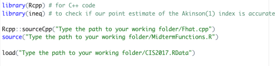
Make sure the following packages are installed on your version of R: (1) Rcpp and (2) ineq. You can do this by taping this in your R Console:

If one of these commands return a FALSE value then install the package using

Make sure you save the C++ function Fhat.cpp that I have created for you in your working directory. This function gives an estimate of the empirical distribution function at each point of the data set of interest. Since it involves n ± n operations, it will save you some cpu time to run it in C++. It is coded for you, you only need to call the function in R as any other R function. The function has only one argument which is a matrix. The first row of the matrix should contain all income observations yi (i e {1, 2, . . . , n}) and the second row of the matrix should contain the vector of associated statistical weight wi (i e {1, 2, . . . , n}). The function will return for each observation i, ![]() i =
i = ![]() (yi). This function will be useful when you will build the Lorenz curves.
(yi). This function will be useful when you will build the Lorenz curves.
Your Midterm.R script should start with
For each question, I will tell you if your script should be in MidtermFunctions.R or Midterm.R
Problem 1: Inequality rankings (45 marks)
In the ineq R library, the Atkinson function generates the point estimate of the Atkinson index without its estimated variance and without accounting for survey weights. The objective of this problem is to create a function Atkinson1 that will generate the point estimate and the estimated variance of the Atkinson index for an aversion to inequality equal to 1, accounting for survey weights. Let F (y) be the distribution on income of interest. For this level of aversion to inequality, the expression for the point estimate of the
Atkinson index is
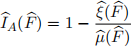
where
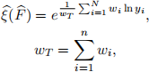
and
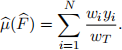
expression of the influence function evaluated at income level yi is

We focus on Eastern Canada in our exam. In your Midterm.R script, create three (3) regions: Atlantic Canada (Newfoundland and Labrador, Prince Edward Island, Nova Scotia and New Brunswick), Qu´ebec, and Ontario. For each region create a 2 ± Nr matrix where Nr is the number of observations for the region. In the first row of each matrix, include the observations of income and in the second row, the associated survey weights. For Ontario, create a vector of 1s of dimension NON .
a) In your MidtermFunctions.R script, create a function called Atkinson1 that is a func- tion of two vectors. The first argument of the function is a vector containing the observations on income and the second argument of the function is another vector containing survey weights (essentially row 1 and row 2 of the matrix of the province). The function should return a vector of two elements. The first element of this vector
is the point estimate of the Atkinson index and the second element is its variance.
(10 marks)
b) In your Midterm.R script, compute the point estimate of the Atkinson index for Ontario using the Atkinson function included in the ineq library (don’t forget to set your parameter to 1 because the default value is 0.5). What is the point estimate?
(5 marks)
c) In your Midterm.R script, compute the point estimate of the Atkinson index for Ontario using your Atkinson1 function assuming that all observation have a weight equal to 1 (use the vector of one that you have created for Ontario as your survey weights). What is the value of this point estimate? How does this compare with the answer in (b). If they are different, you should rework (a). (5 marks)
d) In your Midterm.R script, compute the point estimate and the variance of the Atkin- son index for Ontario, Qu´ebec, and the Atlantic region using your Atkinson1 function. Also construct their 95% asymptotic confidence intervals. What are the values you get? What ranking of these three regions do you get using the point estimates? If you look at their confidence intervals does the inequality between Ontario and Qu´ebec, Ontario and the Atlantic and Qu´ebec and the Atlantic seem statistically different?
(5 marks)
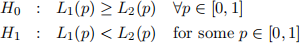
e) Let us now run some statistical tests. We want to test:
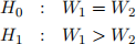
What I will ask you to do here is not 100% accurate. You will run a bootstrap using equal probability sampling but then use the survey weights for computing the statis- tics at each step of the bootstrap. You will proceed similarly each time I ask you to code a bootstrap in this exam. In your MidtermFunctions.R script, create a function called boot.Atkinson that is a function of two matrices and a scalar. The first matrix
is the 2 ± N0 matrix of the region 1 (data1) and the second matrix is the 2 ± N1 matrix of the region 2 (data2). The scalar is the number of bootstrap repetitions.
(10 marks)
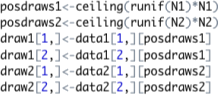
A useful hint: If you want to sample with replacement use the following commands to create the bootstrap samples 1 (draw1) and 2 (draw2):
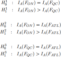
f) In your Midterm.R script, compute the p-values with 999 bootstrap replications, p0 , p1 , and p2 for the following tests: (5 marks)
g) What can you conclude on inequality comparisons between Ontario, Qu´ebec and the Atlantic region. (5 marks)
Problem 2: Lorenz dominance (55 marks)
a) In your MidtermFunctions.R script, create a function named LorenzCoordinates that generates the Lorenz curve coordinates. This function has three arguments: incomes, survey weights, and grid size (hint: since you want to include the coordinate L(0) = 0, it is useful to work with g + 1 as the real grid size and grid size, g as the number of points other than (0, L(0))). This function should return a vector of size g + 1 of the values (![]() (0),
(0), ![]() (p0 ),
(p0 ), ![]() (p1 ), . . . ,
(p1 ), . . . , ![]() (pg e0 ),
(pg e0 ), ![]() (1)). The expression of the estimator of these coordinates is
(1)). The expression of the estimator of these coordinates is
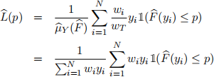
This is where the Fhat.cpp function will help you to estimate ![]() (yi) =
(yi) = ![]() j30(N) wj✶(yj < yi) for each observation. This involves N ± N simple operations (this is more than 80 million operations for Ontario alone) at each step of the bootstrap in the following subquestion. A compiled language such as C++ outperforms an interpreted language such R in doing this. (10 marks)
j30(N) wj✶(yj < yi) for each observation. This involves N ± N simple operations (this is more than 80 million operations for Ontario alone) at each step of the bootstrap in the following subquestion. A compiled language such as C++ outperforms an interpreted language such R in doing this. (10 marks)
b) In your MidtermFunctions.R script, create a function named boot.LorenzCoordinates that will bootstrap the function created in (a). This function has four arguments: incomes, survey weights, grid size and, number of bootstrap replications. This func- tion should return a matrix of 3 rows and g + 1 columns. A first row contains the estimated values of the Lorenz curves coordinates from the original sample, (![]() (0),
(0), ![]() (p0 ),
(p0 ), ![]() (p1 ), . . . ,
(p1 ), . . . , ![]() (pg e0 ),
(pg e0 ), ![]() (1)) (same values as in (a)). The second and third row contain respectively the lower and upper bounds 95% confidence interval of these coordinates. Some will use the 2.5 and 97.5 percentiles of the bootstrap. Many pre- fer to use
(1)) (same values as in (a)). The second and third row contain respectively the lower and upper bounds 95% confidence interval of these coordinates. Some will use the 2.5 and 97.5 percentiles of the bootstrap. Many pre- fer to use ![]() (p) · 1.96 ± σB (p), where σB (p) is the estimated standard deviation for coordinate L(p) in the bootstrap. Since we are assuming a Gaussian process, the last option is better and easier to use. (10 marks)
(p) · 1.96 ± σB (p), where σB (p) is the estimated standard deviation for coordinate L(p) in the bootstrap. Since we are assuming a Gaussian process, the last option is better and easier to use. (10 marks)
c) In your Midterm.R script generate three figures. Each one of the figures displays the line of perfect equality and the Lorenz curves of regions 1 and 2 generated with a grid of 51 points (inclusive of 0) and their 95% confidence bands with 999 bootstrap replications. The list of regional comparisons for these three figures is
(i) Ontario VS Qu´ebec (ii) Ontario VS Atlantic
(iii) Qu´ebec VS Atlantic
(10 marks)
![]() d) What are the rankings suggested by visual inspection of these figures. (5 marks)
d) What are the rankings suggested by visual inspection of these figures. (5 marks)
e) In order to test the rankings obtained by our visual inspection, we have to run a statistical test. This test on Lorenz curves is the following:
If ![]() 0 and
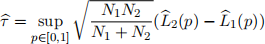
0 and ![]() 1 are the estimators of L0 and L1 respectively, it is straightforward to construct a directional KS type test statistic
1 are the estimators of L0 and L1 respectively, it is straightforward to construct a directional KS type test statistic
The bootstrap procedure to implement this test runs as follow:
1) Repeat for b = 1, . . . , B
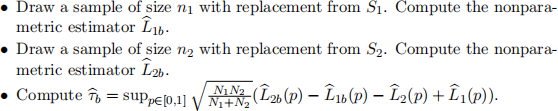
2) Using the sample ![]() 0 , . . . ,
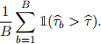
0 , . . . , ![]() B , compute the bootstrap p-value
B , compute the bootstrap p-value
In your MidtermFunctions.R script, create a function named test.Lorenz to run this bootstrap test. This function has four arguments: two matrices and two scalars. The first matrix is the N0 ± 2 matrix of the region 1 (data1) and the second matrix is the N1 ± 2 matrix of the region 2 (data2). The first scalar is the Lorenz curve grid size g and the second scalar is the number of bootstrap repetitions. (10 marks)
f) As usual, the dominance test has a H+ of dominance. Propose an empirical procedure to tests for Lorenz dominance similar to the empirical procedure for stochastic domi- nance presented in class (don’t forget that in Lorenz dominance, the dominant curve is above and in the stochastic dominance case, it is the opposite). In your Midterm.R script, run this empirical procedure on a grid of 51 points for Lorenz curves and 999 bootstrap replications for the following comparisons:
(i) Ontario VS Qu´ebec (ii) Ontario VS Atlantic
(iii) Qu´ebec VS Atlantic
What are the empirical conclusion you reach. Interpret their meaning in term of inequality and compare with the rankings suggested by visual inspection of figures in (d). (10 marks)
2022-02-10