Hello, dear friend, you can consult us at any time if you have any questions, add WeChat: daixieit

PHAS0061 Problem Sheet 2

1. We shall design a Metropolis Monte Carlo procedure to evaluate the canonical statistical prop- erties of a harmonic oscillator when coupled to an environment at a given temperature.

(a) First, let’s do the calculation analytically. The potential energy of the particle is E (x) = κx2 /2 where κ is the spring constant and x is the displacement of the particle from its rest position.  Calculate the canonical mean and variance of the dimensionless displacement x/   = x[κ/(kT)]1/2  where T is the environmental temperature and k is the Boltzmann constant.

(b) The trial changes in configuration are positive or negative shifts through ∆x/  in dimen- sionless displacement. Some attempted shifts are guaranteed to be accepted: which ones?

(c) The other category of shift is to be accepted only on occasion. How would you implement acceptance?

(d) Does it matter what you choose for the initial displacement?  Does it matter what value of ∆x/  is chosen?

2. Using a package of your choice (e.g.  Mathematica, Matlab, python, Excel), implement the Monte Carlo procedure just described and compare the numerically generated expectation value of x/2  with the analytic result.

3. Download and run one or more of the java simulation tools from the PHAS0061 moodle site and generate something numerically that I might find ‘quite interesting’. Bear in mind that my ‘being quite interested’ threshold is extremely low!

4. We shall solve Liouville’s equation for a simple harmonic oscillator in one spatial dimension.

(a) For the Hamiltonian H = p2 /(2m)+κx2 /2 construct the appropriate Poisson bracket and write down the Liouville equation for (∂ρ(x, p, t)/∂t)α,夕 .

(b)  Starting from

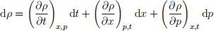
show that

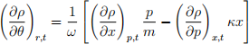
having introduced (r, θ) coordinates through x = κ-1/2r sin θ and p = m1/2r cos θ, and with ω = (κ/m)1/2 .

(c) Assuming a separable solution ρ(r, θ, t) = R(r)A(θ, t) show that

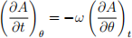
and starting from  to prove that A is a

function of y = θ 一 ωt only.  Interpret this result.

(d) If ρ(x, p, t = 0) is a narrow 2d gaussian centred at (p, x) = (p0 , 0) with p0  > 0, sketch the contours of ρ in the (p, x) phase space at t = π/(2ω). Will the system relax to a stationary pdf as t → &?