Empirical Finance: Methods and Applications 2022
Hello, dear friend, you can consult us at any time if you have any questions, add WeChat: daixieit
Assignment 1
Empirical Finance: Methods and Applications
2022
Problem 1 (5 marks)
Suppose we see 5 observations of yi , Di , shown in the table below:

Consider the following linear model:

Suppose we estimate this model on the data above via OLS. Please explicitly find 
![]() Problem 2: 5 Marks
Problem 2: 5 Marks
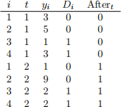
Consider the following difference-in-difference model for individual i in period t e (1, 2}:

Here Di is an indicator variable denoting treated individuals and Aftert is an indicator variable equal to 1 in the 2nd period. Please compute OLS estimates  using the data below:
Problem 3 (10 Marks)
Relative to the United Kingdom, the United States has borrower friendly laws surrounding residential mort- gage default. Many US states are Non-Recourse—that is, if borrowers stop making the mortgage payments, lenders cannot hold them responsible beyond seizing the home itself. On the other hand, the United King- dom has Full-Recourse: lenders may seize cars, investments, garnish wages, et cetera. Many believe that the relative leniency of laws in the United States is responsible for higher rates of mortgage default.
For the sake of simplicity, assume laws may take only two forms: Non-Recourse (in the United States) or Full-Recourse (in the United Kingdom). Imagine we are interested in the causal (treatment) effect of Non-Recourse laws on mortgage default.
(a) Denote mortgage default for a borrower i by Di . In potential outcomes notation, write the average
treatment effect of Non-Recourse laws on default. (3 marks)
(b) Suppose we compare the average default rates in the United States to the average default rates in the
United Kingdom. Write this comparison in potential outcomes notation. (3 marks)
(c) Why does the expression in part (a) differ from that in part (b)? Please provide an explanation that is not simply mathematical, but that provides some intuition. Would you expect the answer in (b) to be higher or lower than that in (a)? Why? (4 marks)
![]() Problem 4 (25 marks)
Problem 4 (25 marks)
In this problem you will simulate and estimate a series of regression models. You should begin by setting a seed in R using the following command: set.seed(123).
(a) Simulate 1000 draws of two independent random variables: vi ~ N(0, 1) and xi(*) ~ N(0, 1).1 Generate
yi as:

where β0 = 1 and β 1 = 0.5. Run a regression of yi on xi(*) . Report your estimates βˆ0 and βˆ1 . (4 marks)
(b) Generate xi = xi(*) + ηi where ηi ~ N(0, 1) is independent of xi(*) and vi . Run a regression of yi on xi . Report your estimate of βˆ1 . Is it meaningfully different from your estimate in part (a)? Explain why or why not. (4 marks)
(c) Rerun the simulations and regressions in parts (a) and (b) 1000 times, saving the coefficients from each iteration.2 Create a histogram of your estimates βˆ1 from the regression in (a) and a separate histogram of the estimates from the regression in (b). (4 marks)
(d) Repeat part (b), but suppose instead that ηi ~ N(0, 10). Maintaining this assumption, rerun the simu- lation and regression from part (b) 1000 times and create a histogram of your estimated βˆ1 coefficients. Are these estimates meaningfully different from your estimate in part (b)? Explain why or why not. (4 marks)
(e) Repeat part (b), but suppose instead that ηi ~ N(0, 0.5). Maintaining this assumption, rerun the simu- lation and regression from part (b) 1000 times and create a histogram of your estimated βˆ1 coefficients. Are these estimates meaningfully different from your estimate in part (b)? Explain why or why not. (4 marks)
(f) Generate y˜i = yi + ei where ei ~ N(0, 1) is independent of yi . Run a regression of y˜i on xi . Rerun the simulation of xi and y˜i and the regression 1000 times and create a histogram of your estimated βˆ1 coefficients. Are your estimates meaningfully different from that in part (a)? Explain why or why not.
Problem 5 (20 marks)
The dataset rollingsales manhattan.xls contains details on 2020 real estate transactions in Manhattan.3 (a) Load the data into R and perform the following basic data cleaning exercises: 4
● Relabel the column names to remove any spaces
– One trick is names(dataset) < _ gsub(” ”, ” ”, names(dataset).
● Remove any observations with the sale price equal to 0.
Using this cleaned data, what neighborhood has the highest average sale price? (4 marks)
(b) Create a new variable equal to log(sale price). Create another variable representing the age of the
property in 2020 (i.e. years since the year it was built). Run an OLS regression of log(sale price) on age and a set of dummy variables for each neighborhood (omitting one). Report the coefficient on age. What does this indicate about the relationship between age and sale price in the sample as a whole? (4 marks)
(c) Run an OLS regression of log(sale price) on age, but use only data from the Upper East Side below 79th street.5 Report the coefficient on age. What does indicate about the relationship between age and sale price in this particular neighborhood. (4 marks)
(d) Plot the mean and median sale price and the total quantity of sales across months in 2020. This can be on multiple figures or a single figure, and you may choose the plotting style that you feel best presents the data. Please comment on and discuss any major patterns you see in these plots. (4 marks)
(e) Create a chart showing a new (and hopefully interesting) pattern of your choice using this data. This
may be a plot of any type, and may relate to the sale price or not. Please briefly describe the plot you have created. (4 marks)
Problem 6 (15 marks)
Disclaimer: this question uses techniques introduced in week 4, so you may want to wait before beginning.
On insendi you will find two data files: regularization train.csv and regularization test.csv. Each contains a single y variable and 50 x variables labeled x1 , x2 , . . . , x50
(a) Set the seed using set.seed(1234). Use cross validation (with 10 folds) to choose λ for a LASSO regression
of y on all x1 , x2 , . . . , x50 . Report the following: (5 marks)
1. The value of λ that minimizes the cross-validated error.
2. The largest value of λ that provides cross-validated error within one standard error of the minimum
3. The number of non-zero coefficients in the model estimated with λ from part 2.
4. The mean squared error from an out of sample test of the model using the testing data regulariza- tion test.csv (again using λ from part 2).
(b) Repeat the exercise in part (a) using 20 fold cross validation. (5 marks)
(c) Repeat the exercise in part (a) using elastic-net with α = 0.1. (5 marks)
Problem 7 (20 marks)
Create a single compelling plot of your choice using financial data and ggplot.
● You must download or otherwise acquire some financial or financially relevant data. This may be from Bloomberg, an online provider (e.g. Yahoo Finance or fred.stlouisfed.org), or any other source.
● Your plot should demonstrate an interesting stylized fact. This could be, for example, the short run price response of an asset or group of assets to some salient event, long run changes in investor flows, or anything that you find exciting. Please be creative and try to identify something that I or your classmates might find interesting.
● Each student must perform this task individually. You are responsible for acquiring data yourself. You may not use data that has been downloaded by a classmate and you may not produce the same plot as a classmate.
● Your answer to this question should cover a single page. The top half of the page will contain the plot, the bottom half will contain an explanation of the stylized fact. Feel free to supplement with regression analysis or other support from the data.
● Your graph will be judged on clarity. Pay attention to labeling and scaling.
● I will select a few interesting plots to present and discuss in class (with permission of the authors).
2022-02-07