STAD70 Statistics & Finance II 2021
Hello, dear friend, you can consult us at any time if you have any questions, add WeChat: daixieit
STAD70 Statistics & Finance II
Assignment 1
2021
Include your codes in your submission.
1. (Normal mixture)
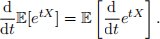
(a) Recall that the moment generating function (mgf) of the standard normal distribution
N (0, 1) is

where X ~ N (0, 1) and t e R. Use this result to show that the kurtosis of N (µ, σ2 ) is 3 for any µ e R and σ > 0. Hint: You may differentiate (repeatedly) under the integral sign, e.g.
Then evaluate at t = 0.
(b) One way of modelling fat-tailed distributions is to use |à|枥│己 枥áz≠a|┐ψ. Given two normal distributions N (µ1 , σ 1(2)) and N (µ2 , σ2(2)), a normal mixture (with two compo- nents) has density

where φ(x; µ, σ2 ) is the density of N (µ, σ2 ) and 0 s λ s 1.
Assume µ 1 = µ2 = µ. Compute the kurtosis of the distribution in terms of the parameters.
(c) Let µ 1 = µ2 = 0, σ 1 = 1, σ2 = 4, and λ = 0.05. Simulate n = 50000 samples from the corresponding normal mixture. Plot the density estimate pˆ(x) together with the theoretical density p(x).
(d) For the distribution p in (c), compute (numerically) the 5% quantile, and compare it with that of the normal distribution whose standard deviation matches that of p.
2. (Relative entropy and excess growth rate) Given two positive probability vectors p = (p1 , . . . , pn) and q = (q1 , . . . , qn) (i.e., pi, qi > 0 and pi = qi = 1), define the |┐己│≠á"┐ ┐|≠|à)5 H(pllq) by
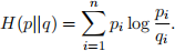
(a) Using Jensen’s inequality, show that H(pllq) > 0 and equality holds if and only if
p = q. Hint: Think of H(pllq) = -Ep ←log ![]() ← where X ~ p.
← where X ~ p.
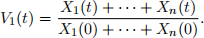
(b) Suppose there are n assets. At time t, t = 0, 1, . . ., let Xi(t) > 0 be the value of asset
i. Consider a buy-and-hold portfolio whose value at time t is
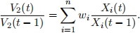
Let V2(t) be the rebalanced portfolio with weights w = (w1 , . . . , wn), where w is a positive probability vector. That is, we have
Let 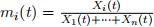 be the capitalization weight of asset i. Show that for each
t we have
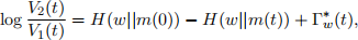
where Γw(*)(t) is the cumulative excess growth rate of the rebalanced portfolio up to time t.
(c) Consider the stocks Ford (F), JPMorgan (JPM), IBM (IBM) and Coca-Cola (COKE). Consider monthly stock prices from Jan 1, 1990 to Dec 31, 2021. Normalize the prices so that the beginning value Xi(0) is 1 and m(0) = (![]() ,
, ![]() ,
, ![]() ,
, ![]() ). Let w = (0.1, 0.2, 0.3, 0.4) (in the same order). Compute the performance of the two portfolios and illustrate the decomposition (0.1) with a figure (similar to Figure 2.6 in the notes). Comment on the results you get.
). Let w = (0.1, 0.2, 0.3, 0.4) (in the same order). Compute the performance of the two portfolios and illustrate the decomposition (0.1) with a figure (similar to Figure 2.6 in the notes). Comment on the results you get.
3. Consider the 4 stocks in Problem 2 (c). Now, consider the sample period Jan 1, 2000 to Dec 31, 2021.
(a) Compute the sample skewness and sample kurtosis for the log returns at daily, weekly
and monthly frequencies (similar to Figure 1). For each asset-frequency pair, perform the Jarque-Bera test and report the p-values. Also compute the autocorrelation (lag 1) for the log return and absolute value of the log return (similar to Table 2). Comment on the results.
(b) Illustrate the aggregational Gaussianity property using one of the assets with (i)
kernel density estimates (similar to Figure 3.4) and (ii) normal q-q plots. Comment on the results.
4. Consider weekly log returns of the FTSE 100 index from Jan 1, 2000 to Dec 31, 2015. Leave the last 80 observations for testing; these observations are not used for fitting the model.
(a) Fit an ARMA model to the data. Explain carefully how you arrive at your chosen
model. Estimate the parameters and examine the residuals.
(b) We examine the out-of-sample performance of the model. Suppose your fitted ARMA model in (a) has order (p* , q* ). For each time t of the testing period, use the data up to time t to fit an ARMA(p* , q* ) model (note that here the order is fixed), and let
rˆt+1|t be the forecast of the log return rt+1 computed at time t. Compute the sum of squared errors
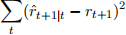
![]()
![]() and compare it with
and compare it with  where r is the sample mean in the training period.
Comment on the results.
2022-01-28