CSCC11 Introduction to Machine Learning, Winter 2022
Hello, dear friend, you can consult us at any time if you have any questions, add WeChat: daixieit
CSCC11 Introduction to Machine Learning, Winter 2022
Assignment 1
This assignment makes use of material from the first 3 weeks, but much of it can be completed after week 2 (Chapters 1-4 of the course note). It includes both written work and programming (in Python). To begin the programming component, download a1.zip from the calendar page on the course website. When you untar the file a directory A1 is created. Please do not change the directory structure, nor the headers of the Python functions contained therein. Please read the assignment handout carefully. Instructions for electronic submission are included below.
We prefer you ask questions on Piazza. Otherwise, for your first point of contact, please reach out to your TA, Zhi Ping (Jacky) Zhuang, through email: [email protected].
1) Written Component
1. Consider Least-Squares (LS) basis function regression for a 1-dimensional input/output problem, i.e.,
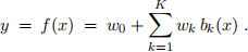
Let the training data be denoted by 
(a) Please formulate the LS objective in terms of a vector of known inputs, a corresponding vector
of known outputs, and the appropriate matrices. Remember to include a bias term in the model (incorporated into the basis function matrix and the weight vector). Note: Please put the bias related terms as the first element/row/column of the vector/matrix.
(b) Then show each step of taking the gradient of the objective function. Note: You may use the matrix identities handout on the course website.
(c) Then solve for the optimal weight vector w (which includes the bias w0).
(d) Suppose now we have a D-dimensional input (i.e. x ∈ RD) and we have set K = 2. How would you define the basis function matrix? How many parameters would you have?
2. Consider again a one-dimensional input/output regression problem. In the following question, we wish to fit a linear regressor and a radial basis function (RBF) regressor, and compare their differences. Recall that a linear basis is f(x) = wx + b and a RBF basis is 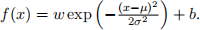
(a) Consider a three-points training set:  = {(0, 1), (1, 1), (2, 1)}. Let µ = 1 and σ =
0.01. What are the optimal parameters for the linear regressor and the RBF regressor? Do they perfectly fit the data?
(b) Unfortunately, measuring data is often a noisy process. Consider now a three-points training set that was collected using a mal-functioned sensor:  =1 = {(0, 1), (1, 10), (2, 1)}. Again, let µ = 1 and σ = 0.01. What are the optimal parameters for the linear regressor and the RBF regressor? Which model fits better? Why?
3. In the following problem we consider cases in which the basis regressor is not well constrained by the data alone.
(a) Assume that you have at least one data point, N ≥ 1. In general, under what conditions will the solution to the normal equations in Q1(c) not be unique? Set up and provide a simple regression problem where the optimal weight vector (w) is not unique.
(b) Consider L2 regularized regression (a.k.a. ridge regression), which adds a term to the LS objective that penalizes the squared L2 norm of w, scaled by a positive regularization parameter λ (see Eqn (10) in Chapter 3 of the online notes). Use the gradient of this regularized objective to derive the normal equations for the solution in this case, and explain the way in which this regularization helps overcome the problem above when the data alone do not fully constrain the solution.
(c) Show that the solution for regularized regression in part (b) can alternatively be obtained via (or- dinary) least squares regression with augmented basis function matrix Bˆ and known outputs ![]() as defined below:
as defined below:

where B is the basis function matrix and y is the vector of known outputs in Q1. IK+1 represents the identity matrix in R(K+1) ×(K+1) and 0K+1 is a zero vector in R(K+1). Note that the quantities inside brackets are block matrices. Explain in short how the above formulation constrains w.
Coding Component
Software requirements: Setup and use the virtual environment following the instructions posted on Quercus.
2) Least-Squares Polynomial Regression
Preliminary. Familiarize yourself with linear regression. Get the demo regression code from the course website. Run the demo, cell by cell. It shows a couple of ways to solve linear least-squares problems, first for
scalar input and output, and then for two-dimensional inputs. It also shows a solution in matrix-vector form.
Now, let’s access and visualize the datasets. Download and untar the starter file, a1.zip, and look in A1/Q2. Load the training data files in the starter directory into Python. The data files are stored as a dictionary in Pickle format. To read them from file,
1. Run one of Python Shell, Jupyter Notebook, etc.
2. Import the Pickle module (Note the underscore): import pickle as pickle
3. Open the Pickle file and read the content (replacing data.pkl below with the actual file name) with open("data.pkl", "rb") as f:
data = pickle.load(f)
4. You may access the training inputs and outputs with data["X"] and data["Y"], respectively. They are stored as numpy arrays with shape (N,1). These are the N-dimensional column vectors comprising the N training inputs and outputs for the regression problem. We’ll denote them here as

The starter code includes three datasets. Each is generated from a polynomial function of a scalar input x, to which noise has been added. Each dataset comes with a small training set, a large training set, and a test set. Among other things this will allow you to see how different amounts of data affect model fitting.
You can visualize the training datasets. This allows you to get some ideas on which models are potentially get a good fit. You can do this using matplotlib, which generates a scatter plot showing the input output pairs:
1. Import matplotlib’s pyplot module:
import matplotlib.pyplot as plt
2. Plot the points:
plt.scatter(data["X"], data["Y"])
plt.show ()
Once you understand how linear regression works and how to manipulate the given data, you may proceed to the next task. Note that there is no deliverable for the above tasks.
Polynomial Regression. We aim to find LS polynomial models for this problem. Each polynomial is ex- pressed as a weighted sum of monomials, where the largest monomial degree is denoted K.
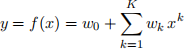
Your goals are to find the LS parameter estimates for wK = [w0,w1,...,wK]T, for each K from 1 to 10. Then, you will select a single model (i.e., find a good value for K). You want a model that will give good predictions on future (unseen) test data. What follows are more detailed instructions. Note: w0 is the bias term and is the first element of the vector wK .
In this section, You need to complete 3 methods in polynomial regression.py. This file contains the class PolynomialRegression with various methods:
1. init (self, K): This is the constructor of the class. K specifies the degree of the polynomial.
2. predict(self, X): This method predicts the output for a given input, using the model parameters. X is a vector of inputs. The method outputs a vector of predicted outputs.
3. fit(self, train X, train Y): This method find the LS model parameters, given training data. train X is a vector of training inputs, and train Y is the vector of corresponding outputs.
4. fit with l2 regularization(self, train X, train Y, l2 coef): This method finds the regularized LS solution. train X is a vector of training inputs, train Y is a vector of training outputs, and l2 coef is the regularization constant, λ, that controls the amount of regularization.
5. compute mse(self, X, observed Y): This method computes the mean squared error between predictions and observed outputs. X and observed Y are vectors of inputs and observed outputs.
Complete the body of the methods: predict, fit, and fit with l2 regularization. Notice that the PolynomialRegression class has the variable self.parameters. It is the column vector containing wK. You will be using self.parameters for prediction, and updating it when performing model fitting (both with and without regularization). Once you have completed PolynomialRegression, you should do some testing to verify your solution! We have provided some basic checks on whether your implementations are correct, but they do not cover all cases. You might want to generate your own noisy polynomial data where you know the ground truth and control the amount of noise.
Written Report. Once you are confident with your implementation, you are ready to explore the ideas of over-fitting, under-fitting, and generalization. In real life, the model that you trained may not perform well in practice. There can be various reasons, but over-fitting and under-fitting are common. You will be learning about what factors contribute to these problems, and what approaches you can use to mitigate them. To this end, the scripts described below will make use of the three datasets provided in the starter code to examine how the results depend on dataset size, model complexity and the regularization constant:
1. compare dataset size.py: Compares training and test error on various training dataset sizes (un- der the same data distribution).
2. compare model complexity.py: Compares training and test error on various degrees of the model polynomial.
3. compare regularization.py: Compares training and test error for various values of the regular- ization constant λ, where λ ∈ [0, 1].
Look at the plots of squared errors on training and test data as functions of dataset size, polynomial degree K, and regularization coefficient λ. The plots will be generated within the dataset directories. Using short and concise paragraphs or bullet points, answer and explain in questions.txt what you can conclude about over-fitting, under-fitting, and generalization. What degree of polynomial was used to generate the data?
3) Image Inpainting with RBF Regression
Suppose you’re given an image with missing or corrupted pixels, like the image above corrupted by red text (Fig1 (2)). Inpainting is a process of predicting the corrupted pixels, for which we’ll use RBF regression.
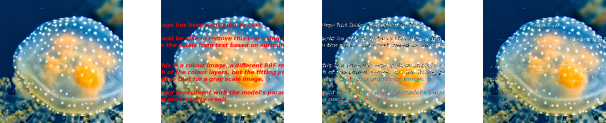
Figure 1: From left to right: (a) The original image. (b) An image corrupted with red text. (c) A badly restored image. (d) A well restored image.
Background: An image is a 2D array of pixels. For greyscale images (Fig2 (left)) each pixel is a scalar, representing brightness. (Color images have three values per pixel, for red, green and blue components, but let’s focus on greyscale for now.) We’ll model an image as a function I(x) that specifies brightness as a function of position x ∈ R2. Pixel values are between 0 (black) and 1 (white).
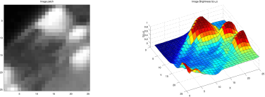
Figure 2: (left) Greyscale image. (right) Depiction of image as a height map where brighter pixels are higher.
We don’t have an equation for I(x) that we can evaluate at the corrupted pixels, but we can use basis- function regression to find one. Because images are smooth and correlated in local regions, we want basis functions that represent the brightness in one region more or less independently of other regions. So let’s use radial basis functions (RBFs); i.e., as in Chapter 3 of the notes, let the model be
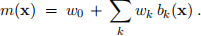
where bk is the kth basis function:

The RBF is a smooth bump centered at location ck ∈ R2 with width σ2. We’ll assume the basis functions are centred on a square grid, all with the same width. You will specify the grid spacing and the RBF width, and then find find the weights wk (including the bias) using regularized least squares regression on image patches. For example, for a 3 ×3 grid of RBFs, with all weights equal to 1, the model might look Figure3left. If instead we use the LS weights (Fig.3middle) we get a better approximation to our image patch (Fig.2right). We get an even better approximation if we use 64 RBFs on an 8 ×8 grid (Fig.3 right). Once we have the model, we can use it to evaluate (or predict) the image values at any pixel (eg. corrupted pixels), or in between two pixels.
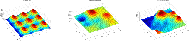
Figure 3: (left) An RBF model with all weight wk = 1. (middle) A model with 3 × 3 RBFs with LS regression weights. (right) A model with 8 × 8 RBFs with LS regression weights. (cf. Fig.2 (right)).
Your Task: The starter code (see A1/Q3) contains methods for handling images. They can crop image patches, reshape the pixels values into vectors of the correct dimensions, and feed these to your regression code. Your task will be to write code to compute the least-squares weights for the RBF model. You will then explore how your model performs for inpainting, varying the RBF spacing, the RBF width, and the regularization constant. The amount of code required is minimal, but it requires an understanding of LS regression, and careful implementation of the right equations. To begin, decompress a1.zip, and look in A1/Q3.
1. Read through the the methods in the starter code. There are two key files, namely, RBF regression.py and RBF image inpainting.py. Pay attention to the examples provided that show how the func- tions are called, and what the expected output should be.
2. Implement 2D RBF regression code. The file RBF regression.py contains the class RBFRegression, along with various methods:
(a) init (self, centers, widths): This is the constructor of the class. In it, centers is a K × 2 matrix that specifies the centers of K RBF basis functions (bumps), and widths specifies a vector of K corresponding widths.
(b) rbf 2d(self, X, rbf i): This computes the outputs of the ith RBF. given a set of the 2D inputs. X is a M × 2 matrix of inputs, where each row (in total M rows) stores a 2D input, and rbf i specifies the ith RBF.
(c) predict(self, X): This method predicts the output for the given inputs, using the model parameters. X is a M × 2 matrix of inputs, where each row (in total M rows) corresponds to a 2D input. The method outputs a vector containing the corresponding predicted outputs.
(d) fit with l2 regularization(self, train X, train Y, l2 coef): This method finds the regularized LS solution. Here, train X is a N × 2 matrix of training inputs, where each row (in total N rows) corresponds to a 2D training input, train Y is a vector of training outputs, and l2 coef is the regularization constant, λ, that controls the amount of regularization.
You should complete the body of the two methods, predict and fit with l2 regularization. Similar to the PolynomialRegression class, the RBFRegression class also has the variable self.parameters. It is the column vector containing wK. You will be using self.parameters
for prediction, and updating it after computing the LS model fit. Again, once you have completed RBFRegression, you should do some testing to verify your solution. The starter code provides some basic checks on whether your implementations are correct, but they do not cover all cases. Remember that your regression code should include the bias term with the RBFs.
You can now run RBF image inpainting.py to remove texts on images. If working correctly and proper hyperparameters, you should obtain a reasonably clean jelly fish (see Fig 1 (d)) with the image Amazing jellyfish corrupted by text.tif. You may also change the settings of RBF image inpainting.py by changing the image, the colour to be filled in, the patch size, similar- ity tolerance, centers, widths, and the regularization constant λ. Examine what happens when you change the distance between RBF centers. What is the effect of RBF width on the reconstruction? What can you say about tuning the model as you increase the amount of hyperparameters? There is no deliverable for this analysis, but make sure you understand how the RBF regression works, and choose appropriate parameters to obtain a clean image.
Submission
1. Written Component
You may hand write or type up (e.g. Word, LateX, etc.) the solutions. We strongly recommend typing it up for legibility. Compile the document as a PDF named A1sol StudentUTORID.pdf (e.g. A1sol student1.pdf). Then you should submit the tar file onto Quercus.
2. Programming Component
Compress the A1 directory into a tar file named A1sol StudentUTORID.tgz (e.g., A1sol student1.tgz). Please don’t modify the method/function headers or the structure of the A1 directory tree since the automarker will fail to run. Failing to follow the instructions will result in a 25% penalty.
To tar and zip the contents, use the command: tar -cvzf name of tar.tgz A1. Make sure to decompress the tar file to ensure the entire A1 directory is there. Then you should submit the tar file onto Quercus.
2022-01-27