Stat 4302 (Spring 2026) Midterm 1
Hello, dear friend, you can consult us at any time if you have any questions, add WeChat: daixieit
Stat 4302 (Spring 2026)
Midterm 1
Academic misconduct It is the responsibility of the Committee on Academic Misconduct to investigate or establish procedures for the investigation of all reported cases of student academic misconduct. The term “academic misconduct” includes all forms of student academic misconduct wherever committed; illustrated by, but not limited to, cases of plagiarism and dishonest practices in connection with examinations. Instructors shall report all instances of alleged academic mis- conduct to the committee (Faculty Rule 3335-5-487). For additional information, see the Code of Student Conduct (http://studentaffairs.osu.edu/csc/).
No form of assistance (from the internet, or from other people) is permitted. You may not discuss this exam with anyone other than your instructor.
Please fill out and sign the form uploaded on the course website, and include it at the beginning of your exam submission.
Please use R for your calculations. Please include any R commands, model output figures, and any interpretations that you make with your submission.
Due by 11:59pm Eastern (Columbus, OH time) on Wednesday February 26. Please submit your exam on the class website.
Please submit two files: 1 pdf file for answers, and 1 file for R code
If you have any questions of clarification, please email me at [email protected]. TA will not answer questions regarding exams. There will be no lecture or office hours while the exam is held.
Question 1 (20 points)
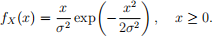
The Rayleigh distribution is a continuous probability distribution defined on nonnegative values.
A random variable (RV) X follows a Rayleigh distribution with scale parameter σ > 0, denoted by X ~ Rayleigh(σ), if it has probability density function (pdf)
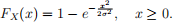
The cumulative distribution function (CDF) for Rayleigh distribution is
Important: You will not receive ANY credit if you use the built-in R functions drayleigh, prayleigh, qrayleigh, or rrayleigh. You must write your own R functions.
(1) (2 points) Write an R function that calculates the pdf for a Rayleigh distribution. Make sure that you add comments to the R code to describe the arguments to the function, and explain how your code works.
(2) (3 points) Using your pdf function in part (1), produce a single plot showing the Rayleigh pdf for σ = 0.5, σ = 1, and σ = 2. The plot must include properly labeled x- and y-axes, a legend indicating the value of σ, and all three curves displayed on the same figure. Based on this plot, describe how the scale parameter σ affects the shape of the distribution.
(3) (4 points) (i) Explain, using mathematics and words, how to generate Rayleigh distributed random variables using the inverse transformation method. (ii) Then write an R function that generates n Rayleigh distributed random variates using this method. Make sure that you add comments to the R code in your function to describe the arguments to the function, and explain how your code works.
(4) (3 points) Suppose X and Y are independent N (0, σ2 ) RVs. Then
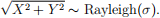
Use this fact, write another R function that generates n Rayleigh distributed random variates. Make sure that you add comments to the R code to describe the arguments to the function, and explain how your code works. [Hint: you may use rnorm to generate random variates from normal distribution.]
(5) (2 points) Using your R functions from part (3) and (4), generate two independent samples of size n = 10,000 from a Rayleigh distribution with σ = 1. Remember to set your seed using set. seed() before simulation; set your seed to the number in your OSU username (for example, if OSU username is cai.1083, then use set. seed(1083)). Print out the first 5 random variates generated by your R function from part (3) and (4). [Note you should print 10 values in total]
(6) (4 points) (i) Produce two histograms of your simulated random variates from part (3) and
(4), respectively. Make sure that the histogram has at least 50 bins. (ii) For each histogram, add the a line representing the true pdf on top of the histogram. (iii) Make a quantile-quantile plot to compare your simulated random variates from part (3) and (4). (iv) Based on your graphical explorations, comment on the simulation performance of your function in (3) and
(4). Explain.
(7) (2 points) (i) Benchmark how long it takes to generate 10,000 random variates using your functions from (3) and (4), and (ii) comment on which method is faster.
In this question, we study a dataset of hospitalizations and intensive care unit (ICU) admissions and occupancies collected from official sources and collated by Our World in Data. Our goal is to assess the rate of ICU occupancy per million people living in the United States during part of the COVID-19 pandemic. High ICU occupancy represents a serious public health concern.
The dataset covid-hospitalizations . csv is available for download on the class website. This is a comma-delimited file that can be read into R using the read . csv function. The dataset contains the following variables:
entity : name of the country (or region within a country)
iso_code : International Organization for Standardization (ISO) code 3166-1 alpha-3 for the country (3 letter country code)
date : Date of the observation
indicator : See description in the following Table of Indicators
value : the value of the indicator
|
Indicator Name |
Description |
|
Daily hospital occupancy |
Number of COVID-19 patients in hospital on a given day |
|
Daily hospital occupancy per million |
Daily hospital occupancy per million people |
|
Daily ICU occupancy |
Number of COVID-19 patients in ICU on a given day |
|
Daily ICU occupancy per million |
Daily ICU occupancy per million people |
|
Weekly new hospital admissions |
Number of COVID-19 patients newly admitted to hospitals in a given week |
|
Weekly new hospital admissions per million |
(reporting date and the preceding six days) Weekly new hospital admissions per million people |
|
Weekly new ICU admissions |
Number of COVID-19 patients newly admitted to ICU in a given week |
|
Weekly new ICU admissions per million |
(reporting date and the preceding six days) Weekly new ICU admissions per million people |
(1) (5 points)
Read the file into R using the read . csv function.
Report the number of variables and the number of observations (in other words, the dimen- sion of the dataset).
Investigate whether any missing values are present and report your findings.
Show the names of all variables, and show the rows of 1234, 18317, 136438, and 193947 of this data frame.
List all countries that are represented in this dataset and report the total number of coun- tries.
(2) (3 points)
Convert the variable date into a “Date” class using function as . Date.
Report the range of observations (in other words, what are the earliest and latest dates in the date frame).
Extract information of year, month, and day from the date variable and store them in new variables, named year, month, and day, respectively.
(3) (3 points)
Create a data frame called US. hosp that contains only observations for the United States; show the first 10 rows of this data frame (US. hosp).
Then create another data frame called US . ICU22 that contains only observations from the United States in year 2022 for which the variable indicator equals “Daily ICU occupancy per million.” Sort US . ICU22 by the variable date in increasing order and display the first
10 rows.
Use the data frame US . ICU22 created in part (3) for parts (4) through (6).
(4) (3 points)
Produce a line plot of the daily ICU occupancy per million versus date in year 2022 (from Jan 1, 2022 to Dec 31, 2022). Add labels for the x-axis and y-axis properly. Add main title as “Daily ICU per million in year 2022 in USA”.
Describe in detail what you learn about the daily intensive care unit occupancy per million people living in the United States from this figure.
(5) (6 points) [Hint: Review Lecture 6]
As is common in statistics, the data variables studied here are measured with uncertainty. Assume that the events of “daily ICU occupancy per million people living in the United States exceeds 20 in 2022” are independent and identically distributed Bernoulli random
variables with parameter p > 0. Estimate the proportion p using the data.
Construct a 90% confidence interval (CI) for this proportion p.
Assess whether there is evidence that p = 0.3, and explain your reasoning.
Assess whether there is evidence that p = 0.15, and explain your reasoning.
(6) (1 point) Consider the assumptions underlying the estimation and confidence interval in part (5). Provide one assumption that is likely violated in this dataset and explain why its violation would invalidate the analysis. [Hint: Review Lecture 6]
2026-03-10