CS 581 Spring 2026 Computational Linkage Design: Part 1
Hello, dear friend, you can consult us at any time if you have any questions, add WeChat: daixieit
CS 581 Spring 2026
Computational Linkage Design: Part 1
Deadline: Thursday, March 5, 11:59pm
Computational Linkage Design is a two part assignment. Part 1 (due March 5) covers linkage design and visualization in matlab. Part 2 (due March 19) involves fabricating a linkage. This document describes requirements for Part 1.
1 Introduction
A linkage is an assembly of bodies connected to manage forces and movement. In this assignment you will design some cool linkages. We’ll only be looking at kinematics and ignoring forces, and furthermore, we’ll limit ourselves to 2D planar structures with revolute joints.
Provided with this assignment is a fully functional Matlab code for simulating linkages. In this assignment you will be responsible for:
1. Modifying the code to allow oscillatory driver input (instead of rotational)
2. Designing several linkages
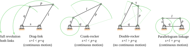
Figure 1: Four-bar linkages. s = smallest link length; l = longest link length; p, q = other two lengths. [image source: wikipedia]
2 Starter Code and Implementation Notes
2.1 Running the Code
Get the starter code linkage.m from Piazza Resources. The provided code is standalone and does not require any external libraries. Here we outline how to run the code from Matlab’s command window:
● Extract linkage.m to working_dir
● Open Matlab and go to the command window.
● >> cd working_dir
● >> linkages(0)
Matlab will then open a figure window that shows the simulation of the sample linkage. The pin constraint between the right and top links is randomized, so if you run the code multiple times, you’ll get a slightly different mechanism each time. The argument “0” specifies the scene to run, which in this case is a crank- rocker mechanism. Each new linkage mechanism that you create should have a new scene number.
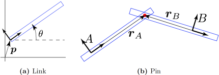
Figure 2: (a) A link defined by its orientation, θ, and position, p. (b) A pin between two links. rA and rB define where the pin location is with respect to the links.
2.2 How to Create Scenes
To create a scene, we need a list of links and a list of constraints between the links. This is done inside the switch statement at the top of the code. The sample four-bar linkage scene is defined in case 0.
Link: A link is modeled as a rigid body, and in 2D, it has three degrees of freedom: θ and p (x, y coords) (Fig. 2a). θ specifies the orientation of the link with respect to the positive x-axis, and p specifies the position of the center of rotation. Given a point, r, in the link's local coordinates, the world coordinates of that point can be computed as
x = R(θ)r + p
where R is the rotation matrix given by
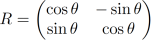
For example, the following code creates a horizontal link at the origin.
links(1).angle = 0;
links(1).pos = [0;0];
links(1).verts = [0,-0.1;2,-0.1;2,0.1;0,0.1]’ ;
The kinematics of a link is fully expressed using θ and p. In order to draw it on screen, however, we need to give it a mesh. In this assignment, we simply assign to each link a list of vertices expressed in the link's local coordinates and transform these vertices into world coordinates whenever we move the link. Note that the mesh is for display only -- the simulation would work just fine even if we don't have a mesh. In the example above, the vertices are
(0, -0.1), (2, -0.1), (2, 0.1), (0, 0.1)
which defines a rectangle with the link's coordinate frame defined at the left end, as in Fig. 2a. These vectors are stored column wise in the links(1).verts matrix.
Additionally, we specify that one of the links is grounded, meaning that it cannot move, and another link is the driver, meaning that its orientation and position are specified procedurally. For example, grounded = 1; driver = 2; specifies that links(1) is grounded, and links(2) is the driver.
Pin: A pin constrains two links with a revolute joint. It stores the indices of the two links to constrain (say A and B) as well as where on the two links the pin constraint is located: rA and rB (Fig. 2b). The constraint should then make sure that, if rA and rB are transformed to world space (using Eq. 1), their locations match. (If you're curious how this is actually implemented, see Sec. 2.2.)
The following code creates a pin between links(1) and links(2) as shown in Fig. 2b:
pins(1).links = [1,2];
pins(1).pts = [4,0;-4,0]’ ;
The links field specifies that the pin is between links 1 and 2, and the pts field specifies that
rA = (4,0) and rB = (-4,0)
Particle: To accentuate the interesting motions of linkages, we can add tracer particles to the links (like the green lines in Fig. 1.) The following code creates a particle.
particles(1).link = 4;
particles(1).pt = [0.5;0.1];
The link field specifies the parent link, and the pt field specifies where on this parent link the particle is located (expressed in the parent link's coordinates).
Hint: When creating scenes, the links do not need to be precisely positioned, since they will snap to configurations that satisfy all the constraints that you specify, as long as those constraints are satisfiable.
2.3 How the Simulation Works (optional reading)
After the scene creation process finishes, we have a list of links, pins, and particles. The simulator then takes this information and does the following:
while simulating
1. Procedurally set the driver angle
2. Solve for linkage orientations and positions
3. Update particle positions
4. Draw scene
end
In Step 1, we manually specify the target angle of the driver link. As long as the mechanism has a single degree of freedom, the orientations and the positions of the rest of the links can be solved for in Step 2 using nonlinear least squares. In Step 3, we compute the world positions of the particles given the newly updated link configurations. Finally, in Step 4, we draw the scene on the screen.
The meat of the simulator is in Step 2. The optimization variables in the nonlinear least squares problem are the orientations, θ , and positions, p, of all the links, including grounded and driver links.
We'll use qi = [θi, pi]T to denote the configuration of the ith link. We are looking for q1 , ..., qn so that all of the constraints are satisfied. There are two types of constraints implemented so far: prescribed and pin. In both cases, we'll express the constraint in the form c(q) = 0.
Prescribed: Grounded and driver links have their configurations manually specified. We can express this as a constraint on the orientation and the position p of the link.
cθ(q) = θ - θtarget, cp(q) = p - ptarget
For grounded links, the target orientation and position are fixed throughout the simulation, whereas for driver links, they are specified procedurally.
Pin: A pin constrains two links so that they share a common point. Let the two links be denoted by A and B. We can express the constraint as
cpin(q; r) = xA - xB = (R(θA)rA + pA) - (R(θB)rB + pB)
We are looking for orientations and positions of the two links such that this constraint function evaluates to zero. The orientations and positions of the two links, θ and p, are the variables of this constraint function, whereas the locations of the pin joints expressed in local coordinates, rA and rB, are the parameters of this constraint function.
Let c be the concatenation of all the constraints. We're looking for the orientations and positions of all the joints (θi and pi) such that the constraint violations are minimized:
minq (1/2) cTc
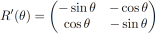
We can solve this easily in Matlab using the function lsqnonlin. What we need to provide is a function that evaluates the vector-valued function c and its Jacobian, J = ∂c/∂q. For grounded and driver constraints, the Jacobian is just the identity: Jθ = 1, Jp = I. For pin constraints, the Jacobian is
J = (∂c/∂θA ∂c/∂pA ∂c/∂θB ∂c/∂pB) = (R'(θA)rA I -R'(θB)rB -I)
where
3 Your Tasks: Linkage Design
3.1 Modify the driver
Modify the driver so that it can also generate oscillatory motion in addition to rotational motion. Currently, the piece of code that produces rotational motion is
...
dt = 0.01;
angVel = 2*pi;
while t < T
links(driver).angleTarget = links(driver).angleTarget + dt*angVel;
...
end
This integrates the target angle with a constant angular velocity (2π radians per second), so that the driver rotates at a constant rate. Your task here is to modify this code so that you can specify a range that the driver oscillates between. For example, if the range is [-π/3, π], then the driver should go back and forth between -π/3 and π at some set frequency. You may not need angVel any more, since the angular velocity will no longer be constant.
3.2 Design a family of four-bar linkages
Four-bar linkages: http://en.wikipedia.org/wiki/Four-bar_linkage. See also Fig. 1. The sample code (linkage(0)) produces a crank-rocker mechanism, since the shortest link, s, is the crank (driver). Copy and paste this sample code and create a
a) drag-link mechanism
b) double-rocker mechanism: the driver motion must be oscillatory, not rotational.
Place all the code in the appropriate case block.
3.3 Design a Hoekens linkage
A Hoekens linkage is a crank-rocker mechanism that produces a nearly straight line from a rotational driver motion. Background information on Hoekens linkages can be found at:
http://en.wikipedia.org/wiki/Hoekens_linkage . Note the figure in the wikipedia page shows a sliding joint that is not required for this assignment. Instead you may follow the mechanism design shown in this video which uses only revolute joints:
https://www.youtube.com/watch?v=2J7P8wHf_gM. Make sure to add a tracer particle to show the trajectory of the tip.
3.4 Design a Peaucellier-Lipkin linkage
The Peaucellier-Lipkin linkage was the first planar linkage capable of transforming rotary motion into perfect straight-line motion, and vice versa. Background information can be found at:
http://en.wikipedia.org/wiki/Peaucellier-Lipkin_linkage. Again, make sure you add a tracer particle to show the trajectory of the tip.
4 Extra Credit
There are two options for extra credit: Designing a Klann linkage (4.1) or extending the current code to allow for pin joints (4.2).
4.1 Klann linkage
The Klann linkage is meant to simulate a walking leg mechanism. Helpful resources can be found at:
● http://en.wikipedia.org/wiki/Klann_linkage
● http://www.mekanizmalar.com/mechanicalspider.html
● https://www.diywalkers.com/klann-linkage-optimizer.html
For this mechanism the geometry of some of the links will no longer be rectangles. You'll need to modify the verts field of link to make this change. Note that the drawScene() function draws the link geometry by connecting the vertices in the order they are defined.
4.2 Pin Joint
The current code only allows for pin joints. For extra credit, implement a sliding joint and design a scissor mechanism [http://en.wikipedia.org/wiki/Scissor_mechanism]. You will have to modify, among other things, objFun(). This function is called by lsqnonlin to evaluate the constraints. To make this modification a little easier, you may want to ask lsqnonlin to use finite differencing instead of using analytical gradients. You can do this by setting ’Jacobian’ from ’on’ to ’off’ in optimset (or optimoptions). The code will be slower with finite differencing, but providing analytical gradients can be tricky business.
5 Submission Instructions (on Gradescope)
5.1 Report
Please provide a report with your submission (PDF). The report should include the following:
● Images: Include images of all mechanisms that you designed. The full path of the tracer particles should be visible. Label each image.
● References: Were there any references (books, papers, websites, etc.), besides the
lecture and lab material, that you used for completing your assignment? Please provide a list.
● Issues: Are there any known problems with your code? If so, please provide a list and, if possible, describe what you think the cause is and how you might fix them if you had more time or motivation. This is very important, as we're much more likely to assign partial credit if you help us understand what's going on.
● Extra Credit: If you did extra credit, include an image of the mechanism. Describe what was done to achieve the linkage design and how you did it.
5.2 Code
Submit your Matlab code. It should run simply by calling “linkages(n)”, where n = 0, 1, 2, 3, ..., is the scene number.
5.3 Grade Breakdown
Computational Linkage Design: Part 1 is graded /80 points, and counts toward 8% of your final grade. The breakdown is as follows:
|
Task |
Max points |
|
Modify Driver |
10 |
|
Four-bar linkage: Drag-link |
10 |
|
Four-bar linkage: Double-rocker |
10 |
|
Hoeken linkage |
20 |
|
Peaucellier-Lipkin linkage |
20 |
|
Report |
10 |
|
Extra Credit (Klann linkage or Pin joint) |
5 |
Remember these assignments are to be done on your own. Do not share code or implementation details with other students.
2026-03-05