Hello, dear friend, you can consult us at any time if you have any questions, add WeChat: daixieit

Fin6116 Fixed Income Securities

Assignment 1

Due date: Mar 04, 2026

1. Which of the following best describes the economic signal of an inverted (downward-sloping) yield curve?

A.  Strong economic growth and rising inflation expectations

B.  Stable short-term rates with neutral outlook

C. Expected economic slowdown or recession, with anticipated future rate cuts

D. High demand for long-term bonds due to fiscal expansion

2. According to the Pure Expectations Theory, what determines the forward rate f(t, t + n)?

A.  The liquidity premium required by investors for holding long-term bonds

B.  The expected future short-term rate plus a risk premium

C.  The market’s expectation of the future short-term rate (no risk premium)

D.  The diference between current short- and long-term yields

3. In PCA-based yield curve modeling, which principal component corresponds to a parallel shift in the entire curve?

A.  Second PC (Slope)

B.  Third PC (Curvature)

C. First PC (Level)

D. Fourth PC (Higher-order twist)

4. What is the primary purpose of bootstrapping in yield curve construction?

A.  To fit a smooth parametric curve (e.g., Nelson-Siegel) to all bond prices

B.  To minimize pricing errors using generalized least squares

C.  To derive zero-coupon discount factors step-by-step,  starting from short-maturity instruments

D.  To interpolate missing maturities using linear regression

5. Which central bank tool involves setting a target for a specific point on the yield curve (e.g., 10-year JGB yield) and buying/selling bonds to maintain it?

A.  Quantitative Easing (QE)

B. Forward Guidance

C. Yield Curve Control (YCC)

D. Interest on Reserves (IOR)

6.  The break-even inflation rate is approximated by:

A. Nominal Treasury yield minus real GDP growth

B.  TIPS real yield minus nominal Treasury yield

C. Nominal Treasury yield minus TIPS real yield

D.  CPI inflation minus nominal yield

7. Which interpolation method ensures continuous first and second derivatives, making it suitable for forward rate estimation?

A. Linear interpolation on yields

B. Linear interpolation on discount factors

C.  Cubic spline interpolation

D. Nearest-neighbor interpolation

8. In the Nelson-Siegel model, the parameter β2  captures:

A.  The long-run asymptotic level of interest rates

B.  The steepness of the curve at the short end

C.  The curvature (hump or dip) in the medium-term part of the curve

D.  The speed of mean reversion in rates

9. Why is the Vasicek model considered a mean-reverting process?

A. It assumes constant volatility across all maturities

B. It uses geometric Brownian motion for rate dynamics

C. Its drift term a(b - rt) pulls the rate toward a long-term mean b

D. It incorporates stochastic volatility via Heston-type terms

10. Which statement correctly contrasts direct (bootstrapping) and indirect (Nelson-Siegel/spline) yield curve methods?

A.  Direct methods are smoother but sufer from model misspecification; indirect methods are exact but noisy.

B.  Both produce identical results when data is perfect.

C.  Direct methods give discrete, arbitrage-free points but may be jagged; indirect meth- ods yield smooth curves but risk model bias.

D. Indirect methods always outperform direct methods in pricing accuracy.

11. We consider the following increasing zero-coupon yield curve:

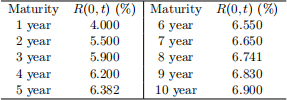
R(0, t) is the zero-coupon rate at date 0 with maturity t.

(a)  Compute the par yield curve.

(b)  Compute the one-year forward yield curve.

12. Open-Ended Discussion Question Compare and contrast Quantitative Easing (QE) and Negative Interest Rate Policy (NIRP) as tools of unconventional monetary policy.

(a)  Briefly explain how QE works to influence financial conditions.

(b) How does QE difer from traditional short-term interest rate cuts in its transmission mech- anism and intended impact on the yield curve?

(c) Which type of interest rate—short-term policy rates or long-term rates—has a more sig- nificant impact on real economic activity (like business investment and housing)?  Explain.

(d) Under what economic conditions (e.g., after a financial crisis, during secular stagnation) should a central bank prefer using QE or NIRP over traditional tools?  Justify your rea- soning.

13. (Optional, with bonus points) Principal Component Analysis (PCA) of Yield Curve Movements

The table below shows the yield (in basis points, bp) for zero-coupon government bonds at 10 diferent maturities over 20 consecutive time periods (e.g., days or months).

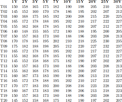
Task: Calculate the yield changes (r) for each maturity and use Principal Component Analysis (PCA) to identify the three key factors (e.g., level, slope, curvature) that explain the majority of the yield curve’s variation.

Instruction:

1. Calculate r: For  each of the  10  maturities,  calculate the yield change  (δr)  between consecutive time periods (T02-T01, T03-T02, ..., T20-T19). This will give you a 19 × 10 matrix of yield changes.

2. Perform PCA: Apply Principal Component Analysis to this 19 × 10 matrix of δr.

3. Interpret the Results:

(a)  Report the proportion of total variance explained by the first three principal compo- nents.

(b)  Plot the ”factor loadings” of the first three principal components against the maturi- ties (1Y, 2Y, ..., 30Y).

(c)  Based on the shape of the loading plots, identify what each of the first three compo- nents likely represents (e.g., a parallel shift in the yield curve, a change in slope, a change in curvature).

14. Bootstrapping and Interpolation

The following bonds are trading in the market:

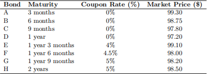
Assume all bonds have a face value of $100. Bonds E through H pay semi-annual coupons.

(a) Bootstrapping: Calculate the zero-coupon yields for the 9-month, 1.25-year, and 2-year maturities using the bootstrapping method.

(b) Interpolation: Using your results from part (a), apply linear interpolation to estimate the:

•  1.1-year zero-coupon yield

•  1.75-year zero-coupon yield

•  1.9-year zero-coupon yield

(c) Validation: Use your interpolated rates to calculate the theoretical price of Bond G (1.75 years, 5% coupon). Compare with its actual market price of $98.2.

(d) Refinements: Now bootstrap the 1.75-year zero rate directly from Bond G and compare it with your interpolated 1.75-year rate from part (b).  Discuss the limitations of linear interpolation for pricing coupon bonds.

15.  From the prices of zero-coupon bonds quoted in the market, we obtain the following zero-coupon curve:

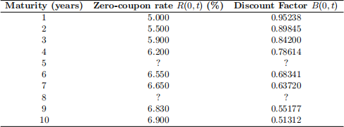
where:

• R(0, t) is the zero-coupon rate at date 0 for maturity t,

• B(0, t) is the discount factor at date 0 for maturity t.

(Hint: you may use R/excel/Python for solving the questions below.

(a) Use linear interpolation with the zero-coupon rates to estimate R(0, 5) and R(0, 8), and the corresponding discount factors, B(0, 5) and B(0, 8).

(b)  Postulate the following form for the discount function (0, t):

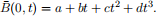
Estimate the coefficients a, b, c, d that minimize the sum of squared errors:

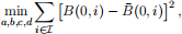
where = {1, 2, 3, 4, 6, 7, 9, 10} is the set of observed maturities.  Then compute:

• (0, 5) and (0, 8),

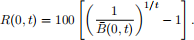
• and the implied zero-coupon rates: