Hello, dear friend, you can consult us at any time if you have any questions, add WeChat: daixieit

R Assignment: Regression Analysis with California Schools Data

Econometrics

Spring 2026

Overview

In this assignment, you will use R to explore key econometric concepts using the CASchools dataset from the AER package. This dataset contains information on 420 K–6 and K–8 school districts in California, including test scores, school expenditures, and demographic characteristics. You will investigate sampling variation, omitted variable bias, and the partialling-out interpretation of multiple regression. At the end, you will produce a professional regression table using the stargazer package and export it to a Google Document.

Deliverables

Submit (1) your R script with all code and (2) a Google Document the figures and regression table, along with written answers to the questions that ask for analysis.

Getting Started

Open RStudio and create a new R script by going to File → New File → R Script. This opens a blank text editor where you will write your code. You can run a line of code by placing your cursor on it and pressing Ctrl+Enter (Windows) or Cmd+Enter (Mac). You can also highlight multiple lines and run them all at once.

Each of the tasks I require you to do in R, I provide code for you to do, making this first assignment not so challenging. I want to give you practice executing code in R, and seeing the econometric concepts we have learned play out with real data.

A lot of the code I have given you has “comments” these are things written after the # symbol appears. I put them in there to describe what is going in with the code to make it easier to comprehend what is happening. They are not necessary for executing the code, in fact the # symbol means to R that it should ignore everything after it.

You will find that it is difficult, to copy paste the code I have given you. That is intentional. I think you will learn more if you type out the commands yourself instead of copy-pasting it. Of course, as I stated previously you are free to use AI to help you with this assignment in any way you wish. My recommendation would be to type out the commands yourself, but then to ask AI to help you understand what the different commands are doing if you are not able to figure it out yourself. Also, if you have errors and things do not work properly, asking AI to help you figure out why could be a good idea.

Begin by copying the following code into your script and running it to load the data and required packages:

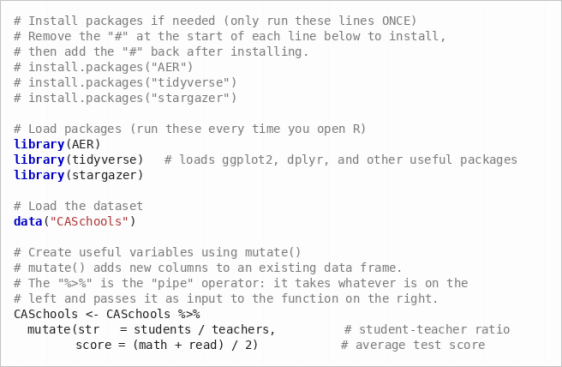
Tip: If you see an error like there is no package called ’tidyverse’, it means you need to install the package first. Remove the # in front of the install.packages() line and run it.

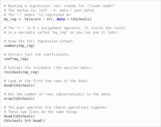
A Quick R Primer

Here are a few essential R concepts you will use throughout this assignment:

Part 1: Sampling Variation in the Slope Coefficient

Suppose the 420 districts in CASchools represent the full population of interest. The “true” pop-ulation regression of average test score on the student-teacher ratio is:

scorei = β0 + β1 · stri + ϵi

(a) Estimate the population regression using all 420 observations. Run the following code:

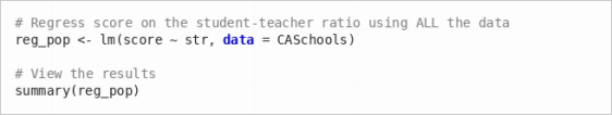
The output from summary() shows a table of coefficients. The row labeled str contains the estimated slope coefficient ˆβ1. The “Estimate” column gives the coefficient value and the “Std. Error” column gives its standard error. Record both of these numbers—you will use them later. Since we are treating the full dataset as the population, this slope is our “true” β1 for this exercise.

(b) Now we will simulate what happens when a researcher only has access to a sample from this population. Run the following code, which draws 105 random districts and estimates the regression on that smaller sample:

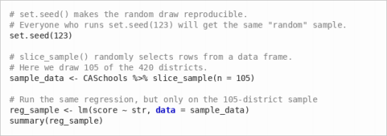
Report the slope coefficient from this sample regression. Is it the same as the population slope from part (a)? If yes, why, if not why not?

(c) Now we will see sampling variation in action. The following code repeats the exercise from part (b) one thousand times: each time it draws a new random sample of 105 districts, runs the regression, and stores the slope coefficient. At the end, we plot a histogram of all 1,000 slope estimates.

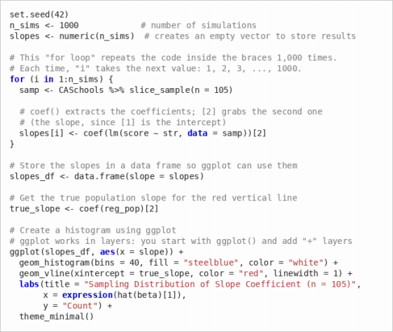
To save the plot: In the RStudio “Plots” panel (bottom-right), click Export → Save as Image or Copy to Clipboard. You can also save it with code by running ggsave("histogram.png") immediately after the plot, which saves the most recent plot as a PNG file in your working directory. Include the histogram in your submission.

Discuss: What does this histogram represent? What does the red line represent? Why aren’t all the slope estimates the same?

(d) Compute the standard deviation of the 1,000 slope estimates:

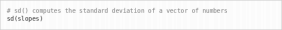
This is an empirical estimate of the standard error of βˆ 1 when n = 105. Now recall that in part (a), you estimated the regression using all n = 420 observations and recorded the standard error from that output. Your empirical standard deviation from the simulation should be approximately double the standard error from part (a). Confirm that this is the case, and explain why. Hint: What is √420/105? How does this relate to the formula for Var(ˆβ1)?

Part 2: Omitted Variable Bias

In the lectures, we saw that the regression of math scores on expenditure per student is confounded by income. Wealthier districts tend to spend more on schools and have students who perform better for reasons beyond school spending (more resources at home, etc.).

We will explore a similar story using the student-teacher ratio (str) as our independent variable of interest and income (district average income in $1,000s) as the potentially omitted variable.

(a) Run the following three regressions:

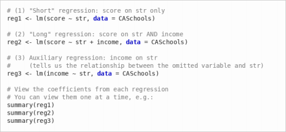
Report the coefficient on str in regressions (1) and (2). How does controlling for income change the estimated effect of the student-teacher ratio on test scores?

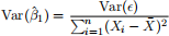
(b) Recall the OVB formula from lecture:

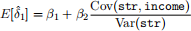
where ˆδ1 is the slope from the short regression (1), β1 is the slope on str from the long regression (2), and β2 is the slope on income from the long regression (2).

The term  is just the slope from regressing income on str—which is exactly regression (3).

Verify the OVB formula numerically using the coefficients you already have. Specifically, show that:

You can check this in R:

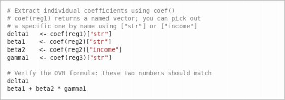
Report the numbers. Do they match?

(c) Discuss: A school board member sees regression (1) and concludes that reducing class sizes (lowering str) will dramatically improve test scores. Why might this conclusion be mislead-ing? What does regression (2) suggest about the true effect of class size?

Part 3: Partialling Out

The “partialling out” interpretation of multiple regression says that the coefficient on str in the regression score = β0 + β1str + β2income + ϵ can be obtained by:

1. Regressing score on income and saving the residuals (the part of scores unexplained by income).

2. Regressing str on income and saving the residuals (the part of the student-teacher ratio unexplained by income).

3. Regressing the residuals from step 1 on the residuals from step 2.

(a) Run the following code to implement the partialling-out procedure:

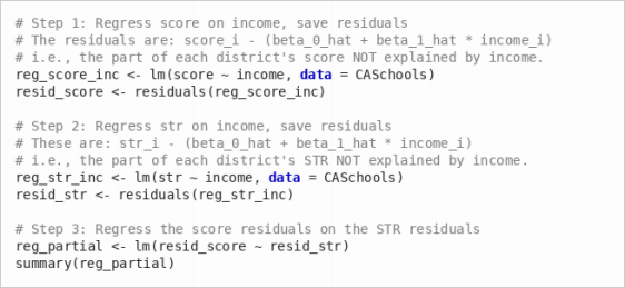
Report the slope coefficient from reg partial. Compare it to the coefficient on str from reg2 in Part 2. Are they the same?

(b) Discuss: In your own words, explain what resid score represents and what resid str represents. Why does regressing one on the other give us the effect of the student-teacher ratio on scores holding income constant?

(c) Create a scatter plot of resid score against resid str with a fitted regression line:

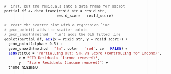
Include this plot in your submission. Discuss: How does this plot differ from a simple scatter plot of score vs. str? What has been “removed” from the data?

Part 4: Regression Table with Stargazer

Now you will create a publication-quality regression table and export it to a Google Document.

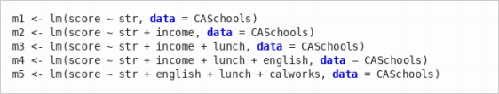
(a) Run the following five regressions. Each one adds additional control variables:

(b) Use the stargazer package to produce an HTML regression table. The stargazer() function takes your regression objects and formats them into a nice table. The argument type = "html" tells it to produce HTML output, and out = "..." saves the result to a file.

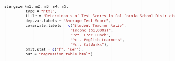
Important: The file regression table.html will be saved in your working directory. To find out where that is, run getwd() in the console. You can change it via Session → Set Working Directory → Choose Directory in RStudio, or by running setwd("your/path/here").

(c) Open the file regression table.html in your web browser (e.g., double-click the file, or right-click → “Open with” → Chrome/Safari/Firefox). You should see a nicely formatted table. Select all the content (Ctrl+A or Cmd+A), copy it (Ctrl+C or Cmd+C), and paste it (Ctrl+V or Cmd+V) into a new Google Document. Give the document a title.

(d) Below the table in your Google Document, write a brief paragraph (3–5 sentences) interpreting the results. Your paragraph should address:

• How does the coefficient on the student-teacher ratio change as you add controls? What does this suggest about omitted variable bias in model (1)?

• Which control variable has the largest impact on reducing the coefficient on the student-teacher ratio?

• Based on model (4), what is your best estimate of the effect of reducing the student-teacher ratio by one student on average test scores, holding other factors constant?