CIVE50003 Computational Methods
Hello, dear friend, you can consult us at any time if you have any questions, add WeChat: daixieit
Computational Methods
Introduction to Structural Analysis Coursework Brief
Lattice structures are commonly used as parts of structural components in a diverse range of engineering fields. They provide an efficient way of spanning planes and volumes using a minimum amount of material. Hexagonal lattice structures are often found in nature perform-ing this role. In 2D a regular lattice structure composed of a single repeating unit, referred to as a unit cell, can be formed from triangles, squares, or hexagons.
When modelling structural components that include lattices it is common, for computa-tional efficiency, to model the lattice using continuum elements that are larger than a unit cell of the lattice. To do this the structural behaviour of a lattice unit cell can be analysed to calculate the apparent material properties of the lattice. Gibson and Ashby’s work in the 1980s examined common lattice structures including regular lattices formed of triangles and hexagons. The linear elastic behaviour of a square lattice structure can be seen to be based on the dimensions of the ‘columns’ and ‘beams’ that form the vertical and horizontal compo-nents of the lattice, when loaded in the x and y directions, while square lattices are prone to shearing when loaded in an off-axis direction.
The aim of this coursework is to consider some of the work of Gibson and Ashby, which was for the most part conducted without the use of computational structural analysis, using a computational implementation of the matrix stiffness method.
Gibson and Ashby demonstrated that the apparent Young’s moduli of lattice structures can be calculated based on the relative density of the lattice structure as:
 (1)
(1)
where Ei* is the Young’s modulus of the lattice for i = 1 or i = 2 (x or y), Es is the Young’s modulus of the solid material the lattice is made from, ρ¯ is the relative density, and α and β are constants depending on the shape of the unit cell the lattice is made from.
The relative density of a lattice can be calculated:
 (2)
(2)
where ρ* is the density of the lattice, ρs is the density of the material the lattice is made from, vs is the volume of solid, and vt is the total volume including voids.
Based on the formulations presented by Gibson and Ashby the theoretical values of α and β for triangles and hexagons in both the x and y directions are given in Table 1.

Table 1: α and β values for triangle and hexagon lattices.
Hunt derives the Young’s moduli of an equilateral triangular lattice structure as:
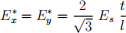 (3)
(3)
Gibson et al. derive the Young’s moduli of a regular hexagonal lattice as:
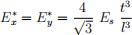 (4)
(4)
where l is the length of each structural member, represented by an edge in the lattice.
The coursework requires you to use the Grasshopper definition that you have developed with the Python component which implements the matrix stiffness method, to carry out structural analysis for two 2D lattice structures, one composed of equilateral triangles, and one composed of regular hexagons. All of the beams forming the lattice structures should have the same rectangular cross-section, with a unit breath of 1 going into the plane, and a thickness t (depth), as required to give relative densities of 0.05, 0.1, 0.15, 0.2 and 0.25.
You are required to calculate α and β for both Ex and Ey, for both lattices, and to compare these to the values given, explaining the reasons for any differences.
For the report you should calculate α and β using the results of analyses carried out for a single unit cell for each lattice. When calculating the relative densities and Young’s moduli of each of the unit cells you will need to take care to consider the appropriate repeating unit for each calculation in the overall lattice structure. You will also need to take care to consider what boundary conditions are appropriate so that the unit cell in isolation behaves as it would when surrounded by other unit cells in a lattice.
You are also required to develop Grasshopper definitions that allow repeating triangular and hexagonal lattice structures, formed of multiple rows and columns of unit cells to be constructed and analysed, with appropriate boundary conditions and loading automatically applied to establish Ex and Ey for relative density values between 0.05 and 0.25, to demon-strate that the values of α and β found for the unit cells are valid for the corresponding lattices. It is recommended when comparing lattice structures that you use an edge length of l = 10mm for the hexagonal lattice and unit cell, and adjust the edge length of the triangular lattice and unit cell so that the triangle and hexagon enclose the same area.
Each group is required to submit a single zip file containing a PDF of their report and Grasshopper definitions used to implement the structural analysis of the unit cells and lattice structures. You may include other Grasshopper or Python files that you consider useful in the zip file, and are required to include a readme.txt file giving a brief description of each file in the zip file, and making clear which Grasshopper definitions can be used to generate and analyse models of the triangular and hexagonal lattices.
You are encouraged to collaborate between groups, without plagiarising. The submitted report and files must be the original work of your group. Only one submission is required per group. Use of AI tools, including large language models is not encouraged, and if they are used, this must be acknowledged at the start of the report.
The report should be clear and concise and must be no longer than 24 A4 pages, with a minimum line spacing of 1.1, a minimum font size of 10 points and minimum margins of 18mm. A sans serif font should be used. The coursework coversheet is not included in the page count. A table of contents is not required. You may include an appendix which is not included in the page count, but this will not be assessed and may not be read, so all important information must be contained within the main report.
The report should include the following sections:
❼ Introduction: This should include a brief discussion of the advantages and applications of lattice structures, and examples of lattice structures, both man-made and naturally occurring. (around 2 pages).
❼ Methods: This should include an explanation of the structural models you develop, following the stages included in the notes. You are not required to explain those stages implemented within any Python scripts that you have been provided with. It should include an explanation of the relationship between ρ¯, l, and t, for each lattice; and an explanation of how you find the Young’s moduli, Ex and Ey, for each lattice, based on the structural behaviour of a unit cell of each lattice structure. (around 6 pages).
❼ Results: This should include results from your analyses finding α and β, for Ex and Ey, for both the triangular and hexagonal lattices, with a brief explanation of the role of the two constants in describing the structural behaviour of the lattices. (around 4 pages).
❼ Discussion and conclusion. This should include further discussion of your results, with relevant figures, including a clear explanation of the structural behaviour of each unit cell and lattice, as well as discussion of other aspects of structural behaviour that you consider of interest, such as buckling behaviour. (around 8 pages).
The Grasshopper definitions should include sufficient explanation that those defining the unit cells can easily be used to get the results in the report, while those defining the lattices should allow for easy identification of input parameters that are expected to be able to be changed, including the numbers of rows and columns of the unit cell in the lattice, relative density, edge length, and the number of elements along each edge. Groups and individual group members may be invited to a viva to discuss their Grasshopper definitions, and all group members are expected to be able to explain how the lattices are modelled in Grasshopper.
It is anticipated that you will spend around 32 hours on the coursework; around eight hours a week for four weeks, including a two hour computer lab tutorial each week. The ratio of marks awarded for the report and marks awarded for the Grasshopper definitions is around 3:1, while they will be assessed alongside each other.
2026-02-14