闪电代写 -代写CS作业_CS代写_Finance代写_Economic代写_Statistics代写_代码代做_IT代写_加急帮助

Hello, dear friend, you can consult us at any time if you have any questions, add WeChat: daixieit

CEM 395

Computers, Graphing, & Curve Fitting Lab Exercise

(25 points)

A. Use of the A/P Labs Computers

1. Right click on Start → File Explorer. This displays the drives, folders, and files on the computer. You should have a Z: drive with your username on it. This is a folder on the AP Labs domain server which will be available to you from any of the AP Labs domain computers. Please store all files in this directory, not on the computer hard drives or on your desktop.

IMPORTANT: Your lab partner will not have access to your directory. A good way to share data with your partner and to have it available to you at home, is to send it to yourself and to your partner by attaching it to an e-mail. NO flash drives allowed!

2. This account will be available to you at least 18 months so you can use it for future courses.

3. Don’t do this now, but in general, when you are finished using an AP Labs computer, right click on Start → Shut down or sign off → Sign off. This will log you off the computer and allow someone else to log on. Turn off the monitor.

4. Using a browser, go to the D2L course website: www.d2l.msu.edu Log in using your MSU username and password.

In the Exercises & Activities Section find the module for Computer, Graphing, & Curve Fitting Exercise. Obtain two data files (File1.txt and File2.xls) and download them and save them to your Z: drive

B. Using Origin to Make Figures

Excel is very useful as a spreadsheet program but it lacks some of the graphing and curve fitting capabilities of Origin. Origin is not great for doing calculations. When doing data analysis and graphing it is most effective to use a combination of the two programs: Excel to do all of the data calculations, and then copy and paste the final values to Origin for curve fitting and graphing.

In this exercise you will take a text (ASCII) file, import it into Excel for data reduction, and then graph it using Origin. The file contains data for a UV-Vis spectrum. The raw data is in %T and the figure should be in absorbance units (AU).

1. The data file is a text file that contains two columns of data. The first column is wavelength (nm); the second column contains the corresponding %T values for spectrum.

2. Open Excel and then use it to Open the File1.txt data file.

You will need to change the File type from Excel Workbook (*.xlsx) to All files (*.*) or you won’t see the text file. This will start an import process and Excel will convert your file to a spreadsheet. Imported files can either be delimited or fixed width. Experiment with the two methods until you have the data separated into two columns; then click finish.

3. Save the data as an Excel spreadsheet by choosing Save As and then selecting Excel Workbook as the file type. This will give the file the *.xlsx extension.

4. Convert the %T data to absorbance units. (Remember? A = -log(T); and note, the expression is in terms of T not %T) This data should go into column 3. If you don’t know how to do calculations with Excel, the TA can show you how.

5. Select column 1 (wavelength data) and hit the Copy button.

6. Boot the Origin program and use the default directory when prompted. Right click in the first column, A(X), of the Book1 window and select Paste. Repeat this process and paste the column of absorbance values into the second column, B(Y), of the Origin Book1 window.

7. Go to Plot → Line → Line. Choose the column containing the X data (independent variable in this case the wavelengths) and the Y data (dependent variable, in this case absorbance) and click OK. (Note: This option should ONLY be used when plotting spectra in which there are many closely spaced data points. When plotting other types of data, use Scatter instead.)

8. The plot will be displayed on the screen. Make your graph look exactly like the one if Figure 1 below . Modify the axes by double-clicking on them and changing the settings under: Scale (From, To, Increment) and Title & Format (Show Axis & Ticks, Major Ticks, Minor Ticks) so that your graph looks exactly like the example (this includes the number of decimal places on the axis numbers which is found under Labels→ Format). Remove the title and legend box by selecting them and hitting the Delete key. Double click on the Axes labels and type in the appropriate text.

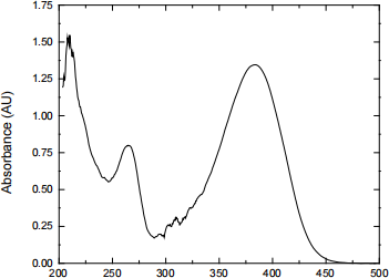
Figure 1: Sample graph of Absorbance vs. Wavelength.

9. Save the project file: File → Save Project, give it a name (keeping the .opj extension) and select your Z: folder to save it in. Origin keeps both the original spreadsheet (Book1) and the plot (Graph1) in one opj file. You can actually have multiple spreadsheets and graphs in one .opj file and rename them to keep track of your work.

10. To copy the graph to a Word document, right click on the plot and select Copy Page in Origin.

11. Open Word. Type your name and the date on the first two lines. Press Enter a couple of times then Paste Special (this is in the Paste dropdown menu on the far left under the Home tab) and select Picture (Windows Metafile). This is important to paste as a picture to keep your file size manageable.

12. Resize the graph to fit the page by dragging a corner. Under the Format tab select the Cropping Tool. Use it to crop (minimize) the white margins on the graph. Deselect the cropping tool and drag a corner to resize the graph to fit on the top of the page. Center the graph on the page and type the figure caption.

13. Save the Word document.

C. Using Origin to Curve Fit Data

The second data file is in an Excel spreadsheet called File2.xls. You will use the curve fitting capabilities of Origin to determine the value of two parameters.

1. Open File2.xls with Excel. Open a new data sheet in Origin (File → New → Project) and paste the data into it.

2. As before, create a graph (this time choose Plot → Symbol → Scatter instead of Line) and scale it appropriately, add labels, etc.

3. When you are satisfied with the appearance of your graph you will curve fit the data to the following equation:

4. To enter a curve fitting equation select Analysis → Fitting → Nonlinear Curve Fit. Select the

Category “User Defined” and for Function, select “New”, which will pop up a new window. You can give the fit a name in “Function Name”, and then click Next. Type in the parameters (a, b, c) in the Parameters box. You will then type in the equation, following the example on the left hand side of the window for the syntax (leave off the “y =” at the beginning). You can change the initial guess for each parameter by double-clicking the numbers under the “Initial Value” column and change it to what you want. In addition to the manual fit, Origin also has a number of predefined fit functions under the other categories.

For example, if you were trying to fit the equation of a line to determine the slope and the intercept:

y = mx + b

you would define the parameters as “m, b” (without the quotes), and then type:

m * x + b

Then, change the Initial Value of m and b to be what you want.

A few tips for the equation above: you need a * whenever you mean multiply and exp(a) is used for ea . Start with initial guesses of a=6, b=1, and c=2. You can check if the equation is typed properly by pressing the running man button under quick check. When you are done entering the equation, click Finish.

5. To actually fit your data to the equation, click Fit. The curve fit line will be displayed on your

graph. If it looks terrible, this indicated that your initial guesses may be bad. Go to the green padlock button on the top left of the plot and select Change Parameters … and then click on Edit Fitting Function (the leftmost square button with pencil picture) to make new guesses (for this exercise, a value of 0.2 for c works much better). After changing the parameters, you need to initialize the fit again by clicking Initialize Parameters and Simplex (P and S with curved arrow) before clicking Fit. You can change the color and shape of the fit line by double-clicking on it and changing the appropriate settings.

6. You’re going to paste this graph and the parameters table onto a second page of the Word

document containing the first graph. To do this, return to the Word document and position the cursor below the caption on the first figure. Hit return a couple of times and then select Insert → Break → Page Break. Hit return a couple of times on the top of page 2 and return to Origin. There is no easy way to copy the parameter table, so you can use Windows’ snipping tool to get the parameter tables and then paste it into the Word document. Return to Origin, delete the parameter table, copy the graph as you did the first graph and paste it on the second page below the parameter table (the parameter table will normally go into the appendix of your report). Again size it to fit the page width and add a caption. Save the file.

D. Using Equation Editor in Word:

Microsoft Word comes with the tool to insert an equation into the line of text. It should come preloaded, but if you are unable to find it please

Whenever you write equations in a document, you should use an equation editor. It is used to write equations and chemical reactions, as well as to create symbols in the text that otherwise cannot be made with Word.

Equations need to be centered on page and numbered at the right. The following instructions will guide you through this process:

1. You will need the “ruler” in Word for this. To always have the ruler on the screen, check the Ruler box under the View tab.

2. In Word, the type of Tab (left, center, right, etc.) is determined by toggling the symbol to the left of the ruler; once the desired Tab type is selected, place the Tab by clicking on the ruler where

you want it. Put a center tab in the center of the page and a right tab at the right side.

3. With the cursor on this line, hit the Tab key and then add an equation by selecting the Insert tab and select Equation (not the pull down just the pi symbol).

4. Type the following equation from the Equation Toolbar. There are a lot of operations so play around-you will need to explore to find the symbols, accents and operations needed for the equation.

Position the cursor to the right of the equation. Hit Tab again and type (1). You should see the following:

(1)

Note that with equation editor in Word, variables are always italicized and that numbers (and functions like sin and log) are not.

5. Chemical formulas and units should not be italicized. When using the equation editor to create chemical reactions or remove italics from the units in an equation, select the text, then Style → Text and the text will not be italicized.

Move down a couple more lines in your document and type the following chemical reaction using equation editor and number it as your second equation:

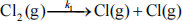(2)

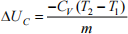
6. Type the following line in your document, using the equation editor for the symbol only:

Since the reaction is exothermic, the enthalpy of the reaction will have a negative value.

E. Page Numbering

1. Number the pages in your document under the Insert tab: choose Page Number → Bottom of Page. Choose Plain Number with bottom center positioning. Select Different First Page (this will only show up under Design when the header or footer is selected); clear the number from the first page, if necessary. Remember how to do this! FYI: When you write a report, you will always leave the number off the first page (the title page); the next page will have a number and it will be page 2. When you are done select the Close Header/ Footer button on the right (or click on the body of the page).

2. At times when writing a report you will want to be able to control where a new page starts. You can do this with a page break. Insert a page break in your document now by selecting Breaks under the Page Layout tab. Choose Page. Your cursor should now be at the top of the second page.

F. Subscripts and Superscripts in Word

Subscript and superscript icons should be in the Font palette on the Home tab. You can also do subscript/superscript by highlighting the text and pressing Ctrl = or Ctrl Shift =, respectively.

Type on the next line:

The symbol for a phosphate ion is .

G. Using Word to Make a Table

1. Position your cursor on a line below the last text in your Word document.

2. Left click on the Insert tab and then click on Table and mouse over to highlight a 3 x 3 Table and click again – it will automatically be inserted into the document.

3. Modify the table to look exactly like the one shown below. First, type the text in the table; then center all the text by highlighting the table and choosing the Center Text icon on the Home tab.

4. Change the column widths by mousing over a column border until the cursor becomes a double line with two arrows. Holding the left mouse button down and moving it will adjust the column width.

5. Mousing over the table will cause a little box to appear at the upper left corner. Clicking on the box will select the entire table. Right-click on the table and select Table Properties from the menu. To center the table on the page; click on the Center icon in the Alignment menu.

6. Cell borders can be changed by highlighting the cell(s), right clicking on the highlighted cell(s), and choosing Table Properties, then Borders and Shading at the bottom of the box. Choose Custom setting and the line Style and then click on the desired line in the Preview box on the right.

7. The angstrom symbol Å can be found by going to Insert tab → Symbol and choosing Font:

(normal text) and Latin 1 supplement- scroll down (it’s a few rows down on the left).

Table 1. Properties of Two Group VIIA Elements