In recent years, Southern California has experienced recurrent wildfire crises, with large- scale fires becoming a near-annual threat across the region.  A stark illustration occurred in January 2025, when wildfires damaged or destroyed more than 9,000 homes and busi- nesses  and  forced  over  130,000  residents  to  evacuate.   Fueled by prolonged drought, intense  Santa Ana winds,  and the  accelerating efects of climate  change,  such events highlight how wildfires have shifted from episodic disasters to a persistent and escalating risk.

Wildfires are not just an environmental emergency - they are a policy challenge.  Pro- environment measures are critical to mitigating these risks and building resilience, but their success depends on voter support.  What makes voters willing to bear the costs of these policies? Does experiencing the devastation of wildfires firsthand change minds?

In this homework, you will investigate whether wildfire exposure makes voters more likely to support costly but necessary pro-environment measures. Using real-world data, you’ll apply the tools of regression analysis to answer a question that lies at the heart of disaster management and climate policy.  This is your chance to connect what you’ve learned so far in the course to a pressing issue facing communities across California, including our own in San Diego.

1    General Instructions

This homework is designed to help you apply the concepts and tools you’ve learned so far to a real-world policy question.  Your goal is to use data and bivariate regression to analyze how exposure to wildfires influences voter support for pro-environment policies.

Here are a few key points to keep in mind:

1.  Focus on Clarity and Interpretation:  The primary objective is to interpret the results of your analysis in the context of the policy question. Explain your findings clearly and concisely.

2. Follow Best Practices in R: Use the coding techniques from lab sessions to manage data, run regressions, and produce clear outputs.

3.  Submission Format:  Submit your assignment electronically through Gradescope (via Canvas). You must upload two files:

•  A clearly labeled R script (LastName PID HW1. R) containing all code used to load data, run analyses, and generate any figures or tables.

• A PDF document containing your responses to all questions,  including written explanations, interpretation of results, figure and table labels, and any required discussion.

Your R script must be well-organized and run without errors.  Assume the grader will download your script into the same directory as the data file.  The script must run as a standalone file from start to finish without any pauses, prompts, or manual intervention.

Before submitting, test your script by running it all the way through in a clean R session.

4.  Collaboration Policy:  You may work with whomever you like, but you must ac- knowledge all collaborators by name in both your written document and your R script.  If you used ChatGPT or any other AI tools for assistance, you must explicitly acknowledge this in your submission.  Your acknowledgment should specify how the tool was used while making clear that you completed the assignment independently.

Example  Acknowledgment  (to  be  included  at  the  beginning  of  your  PDF submission):

ACKNOWLEDGMENTS: For this work, in addition to previous exposure to R programming as an undergraduate Political Science student at UC Santa Barbara, and during QM II lectures, labs, and TA office hours, I, Alexander

J. Norling, acknowledge having worked with my classmates John Doe, Jane Smith, and Alex Taylor.  I also acknowledge having used ChatGPT to trou- bleshoot R code.  Specifically, ChatGPT assisted with resolving errors in data manipulation, enhancing the clarity of my code, and improving the aesthetics of my plots. All interpretations, analyses, and conclusions in this assignment are my own, and I completed this work independently.

This acknowledgment should be included at the start of your PDF document.  Failing to acknowledge collaborators or AI tools constitutes a violation of academic integrity policies.

5.  Submission  Timing and Late Policy:  Homework grades are adjusted automati- cally based on the time of submission, as recorded by the Canvas/Gradescope timestamp:

•  On time:  100% of the earned score.

• Up to 24 hours late: 90% of the earned score (a 10% reduction).

•  After the first day:  the earned score is reduced by an additional  1 percentage point per day late.

For example, an assignment submitted two days late receives 89% of the earned score; three days late receives 88%, and so on.

Because this policy is automatic and built into grading, you do not need to email the instructor or TAs to explain a late submission.  This policy is designed to handle un- expected events consistently and fairly, without requiring documentation or individual appeals.

6.  Ask  for Help:  If you encounter any difficulties, don’t hesitate to reach out during office hours or review sessions.

2    About the Data

The dataset is drawn from the study  “Wildfire Exposure Increases Pro-Environment  Vot- ing within Democratic but Not Republican Areas”, published in the American Political Science Review  (APSR). The original paper examines how proximity to wildfires influ- ences voter support for pro-environment measures.  You can access the full publication here.

For this assignment, you will work with a subset of the dataset focusing on observations from the year 2010 (see wildfire exposure. csv).  Year 2010 is particularly important because it coincides with Proposition 23, a high-profile ballot measure in California that sought to suspend the state’s landmark climate legislation, AB 32.  Voter support for Proposition 23 provides a critical context for understanding the relationship between wildfire exposure and pro-environmental policy preferences.

The unit of observation in this dataset is the Census Block Group (BG), a small geo- graphic unit used by the U.S. Census for data collection. Each row represents a unique BG in California, and the variables capture voter behavior and environmental characteristics.

Key variables include:

• Dependent Variable  (DV): envbi, the Environmental Ballot Index, measures the proportion of votes in favor of pro-environmental policies in each BG.

• Independent Variable (IV): mindist5000, a continuous variable measuring the distance (in meters) from the BG to the nearest wildfire burning at least 5,000 acres within two years before the election.

• Additional Variables:  The dataset includes other variables like voter turnout and precipitation. See the data codebook for additional details on these variables.

3    Your Tasks

Your R script should clearly document the steps you took to complete each task be- low.  Use meaningful comments to explain your code and provide context for each step.

The goal is to ensure that a reasonably knowledgeable person reading your script can understand how you implemented each task and verify your results.  Save your script as LastName PID HW1 . R (e.g., Ravanilla A12345678 HW1. R). Ensure there are no spaces in the filename.

Your PDF submission should include clear answers to all questions (e.g., Q1, Q2, etc.)

listed under each task. Ensure that your answers are well-organized, and any figures or ta-

bles generated as part of your analysis are appropriately labeled and referenced in your ex-

planations. Save your PDF as LastName PID HW1. pdf (e.g., Ravanilla A12345678 HW1. pdf). Ensure there are no spaces in the filename.

3.1    Preliminaries

•  Set your working directory and load the necessary packages in your R script.

• Load the dataset into R.

•  Ensure the variables to be used for the analysis are in numeric format.

• Use the dim() function to determine the dimensions of the dataset.

•  Question 1  (Q1): What do these numbers in the reported dimensions represent in the context of the dataset?

•  Q2: How many observations are in the dataset?

•  Q3: How many variables are in the dataset?

•  Check the dataset for missing values.

•  Q4: How many missing values are present in the dataset?

• If there are missing values in the data, replace them with NA

3.2    Data and Descriptive Statistics

•  Q5:  Which variable would you examine to determine how many BGs were at the center (ground zero) of a wildfire that burned at least 5,000 acres in the past two years?  Hint:  There is more than one possible variable;  you only need to choose one.

• Use the table() function to count the occurrences of each unique value in the variable you selected.

•  Q6: How many BGs experienced a wildfire over 5000 acres in the two years leading up to 2010?

•  Create a new variable called mindistkm that converts the mindist5000 variable (distance to the nearest wildfire in meters) to kilometers.

•  Compute summary statistics such as the mean, variance, and covariance for the dependent variable (envbi) and the independent variable (mindistkm).

3.3    Visualizing the Data

•  Create a histogram for the dependent variable (envbi) to visualize its distribution. Overlay a kernel density curve on the histogram for a smoother representation of the data.  Ensure the figure is clearly labeled with appropriate axis titles and a meaningful title.

•  Generate  a histogram for the  independent variable  (mindistkm)  to  explore the distribution of distances to wildfires,  adding  a kernel density curve.   Label  the axes and add a descriptive title to make the figure easy to interpret.

•  Create a scatter plot with envbi on the y-axis and mindistkm on the x-axis to visualize the relationship between voter support for pro-environment policies and proximity to wildfires.  Add a regression line to highlight the trend between the variables, and ensure the plot is polished with proper labels and a clear title.

•  Save all figures in your working directory using descriptive filenames (e.g., envbi histogram. png or scatter envbi mindistkm. png).

•  Q7: Include the saved figures in your PDF submission.  For each figure, add a note below explaining what the figure shows and its relevance to the analysis.

– What is a Figure Note? A figure note provides context for the visualization, explaining what it represents and why it is important.  It should be concise but informative.

– Example Note:

Figure 1 shows the distribution of envbi, the Environmental Ballot In- dex, across Census Block Groups in 2010.  The histogram reveals  that most BGs have  extremely  low support for pro-environment policies, with  a small cluster of BGs showing very high support.   The  kernel density curve smooths the distribution for easier interpretation.

Hint:  Refer to  Lab  Session Guides for examples of how to create professional-quality visualizations using ggplot2.   Follow the formatting conventions demonstrated in the guide to ensure your figures are clear and well-presented.

3.4    Regression Analysis

• Use the lm() function in R to estimate a bivariate regression model predicting envbi (the dependent variable) using mindistkm (the independent variable).

•  Display  a summary of the regression model.   Include  the  estimated  coefficients (Intercept and mindistkm), standard errors, R2 , and p-values in your output.

•  Save the regression results to a text file using the stargazer package or a similar output tool. Ensure the text file includes a descriptive title and clear labels for the dependent and independent variables.

•  Q8: Based on the regression output:

–  Q8a: What is the estimated relationship between proximity to wildfires (mindistkm) and voter support for pro-environment policies (envbi)?

–  Q8b:  Is the relationship statistically significant?  Justify your answer using the p-value.

–  Q8c: Interpret the R2  value: What does it tell you about how well the model explains the variation in envbi?

• In your R script, “manually” calculate the regression coefficients (b0 and b1) using the ordinary least squares (OLS) formulas:

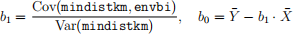
•  Q9:  Compare your manually calculated coefficients with the ones obtained from the lm() function.  Are they identical?  If not, explain why discrepancies might occur.

•  Q10: Explain what the slope (b1) reveals about the relationship between mindistkm and envbi. Specifically, discuss the direction of the relationship, the magnitude (i.e., how much the outcome changes for a one-unit change in mindistkm), and whether the relationship is statistically significant.

•  Q11:  What part of the formula for b1 determines the sign of the slope?  Explain your reasoning.

•  Q12: What does the intercept (b0) represent in this context?